Introduction

Let us start talking about something we all might have used someway or the other, torrents. It works on a peer to peer (p2p) network which is based on an algorithm called Breadth first traversal or BFS.

Consider all the peers are nodes (computer or mobile devices), when a node generates a request message, it is propagated to all its neighbours (other peers), when a peer receives the request it is forwarded to all the peers other than the sender and searches for relevant matches. Hold this thought, this is an overview of how BFS is applied in the real world.

Breadth first traversal is a graph traversal algorithm, exploring all the nodes from a root(source) node to neighbouring nodes. Then it goes to the next nearest node and explores all unvisited nodes, this process is repeated until all nodes are visited.

Basically BFS is a type of graph traversal where nodes of the graph are visited in increasing order of their distance from source node.

For instance, in the graph below the shortest distance between the source node 1 and node 6 will be node1→ node2→ node6.

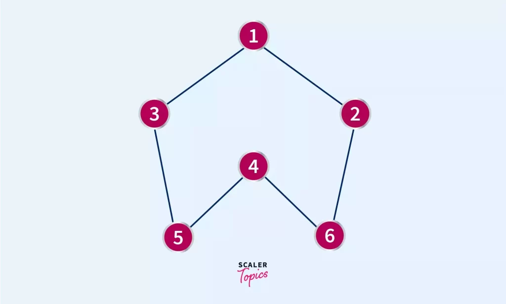
A graph could or could not be a weighted graph i.e. the edges of the graph may or may not have weight, like the graph above did not have weight so the shortest path between nodes will always be the path with least number of nodes visited but in a weighted graph the shortest distance could be a path with more number of nodes visited according to weight comparison, let us see how that looks in picture:

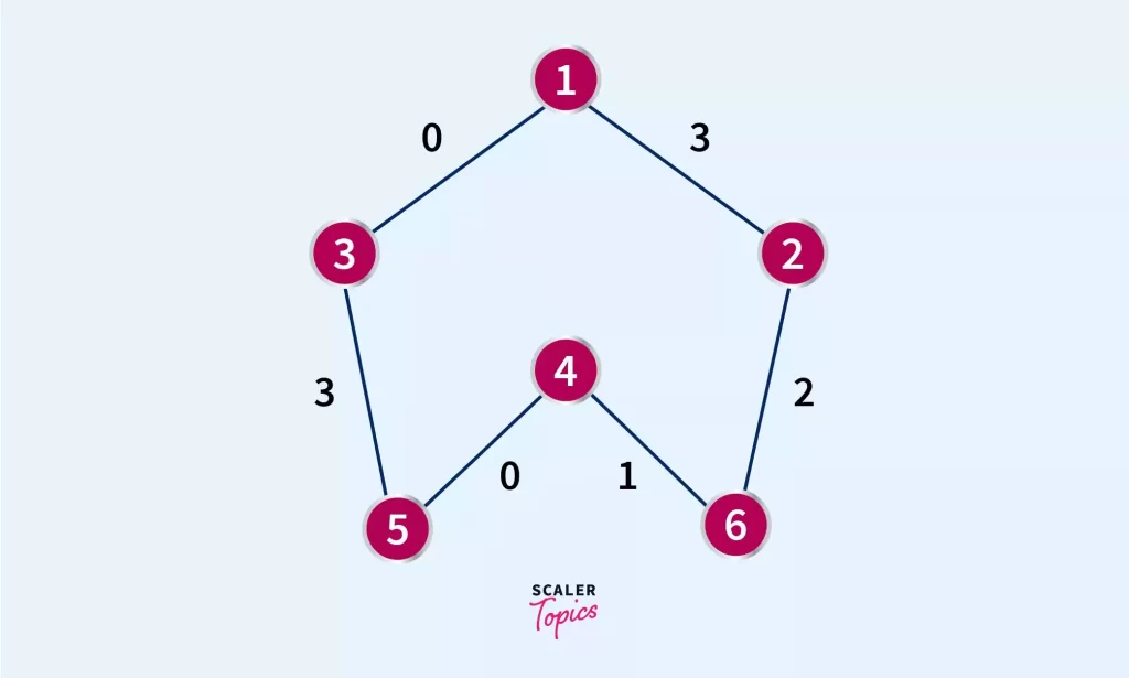
The shortest distance in this weighted graph from source node (1) to node 6 will be :

node1→ node3→ node5→ node4→ node6 as the corresponding sum of weights of their edges is 0+3+0+1 = 4 which is less than node1→ node2→ node6 path (3+2=5). Algos like dijkstra and Bellman-ford are used for weighted graphs but what if edge weights had more constraints.

We still havent talked about the topic of the article, 0-1 BFS, for you all – don’t be anxious, for me – ‘stop beating around the bush’.

These are the constraints I was talking about. If the edge weights are 0 or 1 then we have a smart technique to solve this shortest path problem using a double ended queue (Deque) called 0-1 BFS algo. We’ll find the distance from the source node to every other node and the source node will be known.

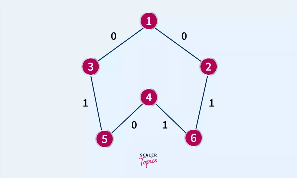
0-1 BFS Algorithm

A vector, d will be defined to store distances between different vertices from source(s). d[s] will be 0 as the distance from source to source is 0. s will be pushed into the front of the deque(q). We’ll visit connected nodes and keep popping the previously pushed node at the front of the queue. We’ll assign u and w as first second edge respectively and push the edge connecting node having weight 0 to front of the queue and if weight is 1, pushing it to back of the queue, this will be repeated till the queue is empty which denotes all the nodes are visited.

Here is basic code of the algorithm:

We’ll understand this algorithm with a pictorial representation of a graph, make yourself a drink, sit back and relax.

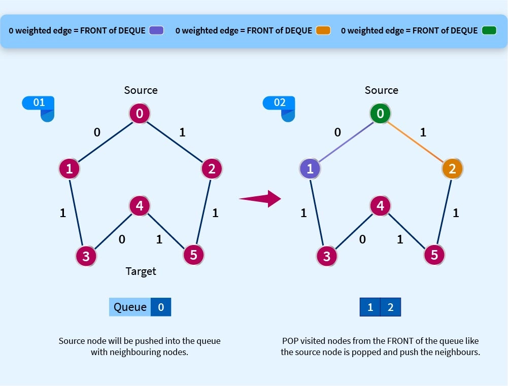
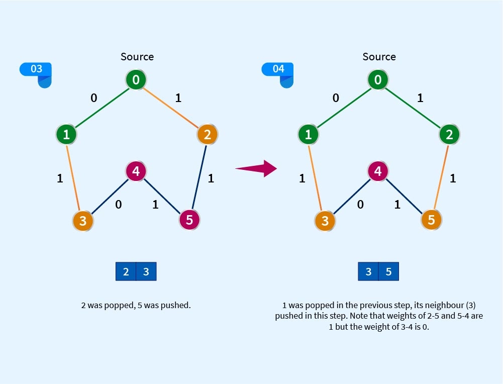
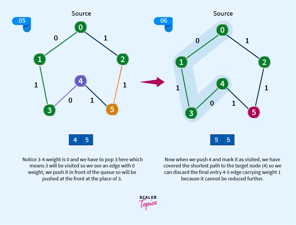
I hope you understand the above representation. It might take a while to grasp, that’s why the drink.

See it’s quite straightforward though, the edge with weight 1 will be pushed to the back of the queue so notice nodes 2,5,4 and 3 were added at the back of the queue as evident from the graph and rest with weight 0 will be pushed in front, the front will always be popped (removed) after being pushed ofcourse and the back element moves to front, but when in the 5th step 3 was popped and due to 3-4 linkage have weight 0 therefore pushed in front.

Now if you completely understand this, I would like us to go through its time complexity.

Suppose a graph G, having V vertices and E edges. It is a weighted graph with boolean weights i.e either 0 or 1.

So while traversing the graph, while visiting a vertex we know we only have two possibilities, an edge having weight 0 or another edge having weight 1, we also know the queue holds two consecutive successive elements (nodes).

So consider if edge weight equals 0 we will push the node to front and if not push it back to end, this allows our queue to remain sorted.

Thus all the nodes are visited minimum once concluding time taken to visit all nodes equals sum of number of edges and vertices. So, Time complexity of 0-1 BFS is O(E + V), which is linear and more efficient than

Dijkstra: O(V2+E) -> (O(E + V Log V)

Example of 0-1 BFS Algorithm

Let us take a complex graph problem as an example, suppose a graph with V nodes and E edges. Edges have binary weights (0 or 1). The source node is the 2nd node and we need to find the shortest path from source node to every other node. Seems sound na. Our logic remains the same, jog your memory with me…We will use double ended queue (DEQUE), because it allows insertion and deletion at the both ends which is exactly what we need:

1. Traverse through all the nodes (first the source node will be pushed in front then its neighbour after popping source)
2. Checking the weight of all the edges
3. Pushing the nodes in the queue, if weight 0 then in front else back of the queue
4. Printing the sum of the weight of edges making shortest path from source node to other nodes

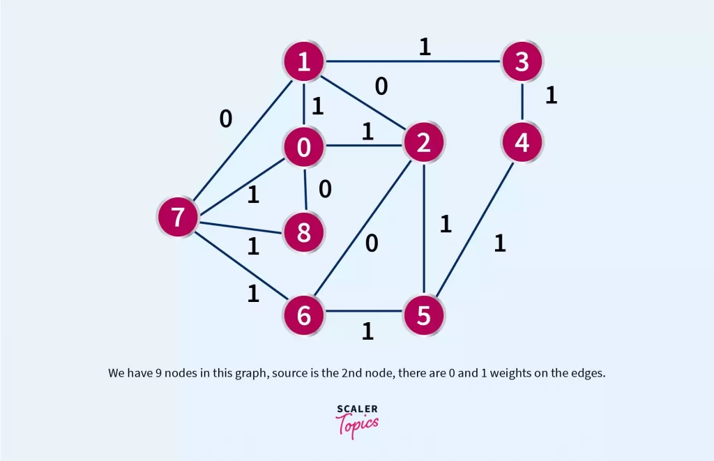
We have 9 nodes in this graph, source is the 2nd node, there are 0 and 1 weights on the edges.

Here is the code for the 0-1 BFS in C++. Above graph is taken as input to the program :

Output

Practice this into a compiler and try manipulating the values if you understand the flow of code, make a graph yourself with pen paper and give edges 0 and 1 weight randomly, put the values in this code, run it and match it.

Read the code and especially the comments with it and understand what action every command is doing.

If you encounter an error google it also sometimes has some issues so try changing the compiler and while checking languages in python make sure to open the python compiler of the required version like python 3 has been used below.

Implementation of 0-1 BFS on Java, Python3

You can find Implementation of above graph problem in Java and Python here:

Java program for BFS

Python program for BFS