Breadth First Search Algorithm (BFS)

Introduction to Breadth - First Search

We have seen how the graphs are represented and how these are useful in representing the connections between the things, e.g. representing a city, where the roads can be thought of as edges and vertices as the houses.

But just like adding or representing the items in the graph, it also becomes important to have some ways we can traverse the graph to iterate over those elements(or Nodes or Vertices).

The transversal is a core part of any data structure, using which we can iterate over all the elements, can search for a particular element, can print those as we traverse, and so on...

In Graphs, there are 2 techniques of traversals, which are Breadth-First Search and Depth First Search.

Breadth-First Search(also known as Breadth-First Traversal) is a traversal mechanism that, as the name might suggest, traverses the graph in a breadthwise manner. This essentially means we start the search from a Node and then explore all of its neighbouring Vertices. Once these neighbouring vertices are explored, then we go ahead exploring all of their neighbouring vertices and so on.

There are a lot of applications of Breadth-First Search when we are dealing with graphs. One of them is to find the shortest path/distance between two nodes of a graph. We start our BFS from one of the two given nodes and explore all of its neighbouring nodes. Now if the second Node is one of these neighbouring nodes, then the shortest distance is 1. Else, we explore the neighbours of all these neighbouring Nodes. If we found the second Node in one of these nodes, then the shortest distance is 2. And so on and so forth.

Now as we know Breadth First Search explores all closer vertices of a node before going down their neighbouring vertices, it guarantees that once we found the target vertex, it's done via the shortest path. This fact is leveraged in many other algorithms and use cases, as we will explore in this section.

Breadth-First Search Example

Before jumping onto the Breadth-First Search, let's recap that the Graph has no root(unlike trees). So we can pick any Vertex of the Graph from and start our Breadth-First Traversal from there.

In the below example we have taken A as the starting vertex(but as discussed above, it could be anything for that matter).

Recall that Graphs can be directed and undirected. Directed graph means if there is an edge from A→ B means we can only go from A to B and not vice versa. But in an undirected graph, if there is an edge between A -- B, then it means the edge is undirected, meaning we can go from A to B and vice versa.

To make things easier, we will be taking undirected graphs only in the below sections. But the only difference in these in terms of Breadth First Search will be that the neighbours may be different.

Example: if it's a directed Graph and we have an edge A → B → C, then neighbour of B is C only. But in the undirected graph of A --- B --- C, both A and C are neighbours of B.

Lets try to understand Breadth First Search with an example graph:

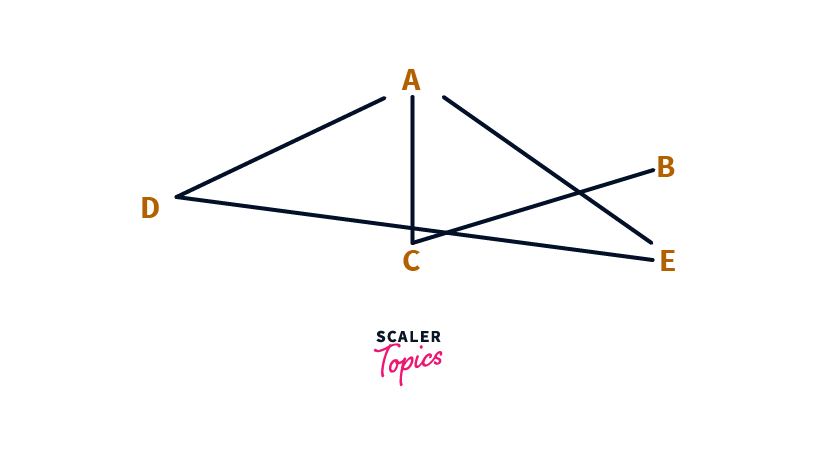
Breadth-First Search focuses on traversing Breadth wise, i.e. we will first traverse all the neighbours of A first, and then explore their neighbours, and so on.

Let's try to clarify this in detail.
As shown, A is connected to D, C, and E directly. So D, C, and E are neighbours of A.
In Breadth-First Search, we will first explore A (as we are starting the BFS from A).
Once A is explored, we need to explore its neighbours i.e. D, C, and E.
When we explore D, C, and E, and look at the neighbours of these nodes we notice that:
Neighbours of D are A and E, but both are already explored, so nothing to do here.
Neighbours of C are A and B. As A is already explored, we ignore it and explore B now.
Neighbours of E are A and D, but again both are already explored, so nothing to do here.

Question: Why are we not exploring the already explored nodes?

Good question, hold on to that. We are going to talk in detail about that below.

Okay, for all the curious readers: it's to avoid cycles(or infinite loops) while exploring. We will talk about this more in the later section.

So we notice that the order we explore the vertices are : A and the D, C, E, and then B. So the order of Nodes in Breadth-First Search of the above graph will be A, D, C, E, B.

This can be summed up in the below figure:

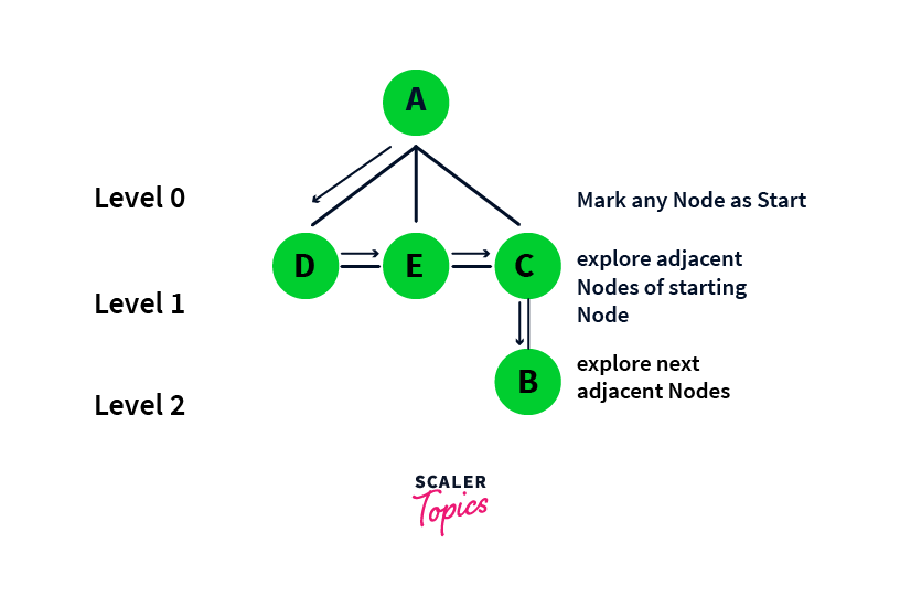
Level: The level can be thought of as the distance from the starting Node, like D, E and C are at distance 1 from A so they have level 1, and similarly, B is at distance 2(as it connects to A via C in between) wrt A.

So as we can see in the above image, we traverse the elements of each level first, before traversing the elements of other levels. Due to the same reason, Breadth First Search can be also thought of as a Level Order Traversal

It can also be noted here that the levels dictate the shortest distance(i.e. Number of edges) between two Nodes. E.g. if we start from A, then D is seen at level 1, so A and D have a shortest distance of 1 between them. Similarly, as B is seen at level 2, A and B have a shortest distance of 2.

So in case if you are ever interested in finding the shortest distance between any two nodes of a graph, Breadth-First Search is your best bet.

You just need to perform a Breadth First Search from one of the two nodes and find the level of the other node. This level will be your shortest distance between those two nodes.

In the below section, we will see how this can be formulated in the form of an algorithm.

Breadth-First Search Algorithm Example

Before jumping onto the Breadth First Search example, let’s understand two important concepts used in Breadth-First Search:

1. Cycles in Graph:

If you might have observed in the above figure, when we are at A, we explore its neighbouring vertices, i.e. D, C, and E. And there are subtle things to care about while doing Breadth-First Search.

When we have explored D, C, and E, we can start exploring D’s neighbouring vertices i.e. A and E. But we have already visited A, so if we go back to A again, it will form a cycle and we will be stuck in an infinite loop exploring A and D and then A again. This is an important point to take care of in the Breadth-First Search.

So to handle such scenarios by preventing the traversal of the same element again, we need to maintain the state of all visited elements.

If we encounter the same element again, which is in that visited data structure(e.g. Sets), we ignore it. This takes care of cyclic traversal problems.

2. Queues in Breadth-First Search:

Another thing to note is that when we are at A, we need to traverse its neighbouring Nodes, i.e. D, C, and E before we can start exploring the neighbours of D, C, and E. Queues are the best data structures that can ensure the element we saw first, will get processed first. Why? Because of its FIFO(First In First Out) property.

Using the FIFO property, we can ensure that the element which was First In (meaning which was First explored and inserted in the Queue) will be First out(meaning will be first to be taken off of the queue to explore its Neighbours).

Using Queues, we can add the element we encountered first, and due to the FIFO property, the element we pick out from the queue(to process) would be the one inserted into it the earliest.

Example
Now let's see how the above points can be used to do a Breadth-First Search from Node A.

Also, as seen above, we need to use two data structures: A Queue queue (for FIFO property) and a Set visited (to mark the visited nodes).

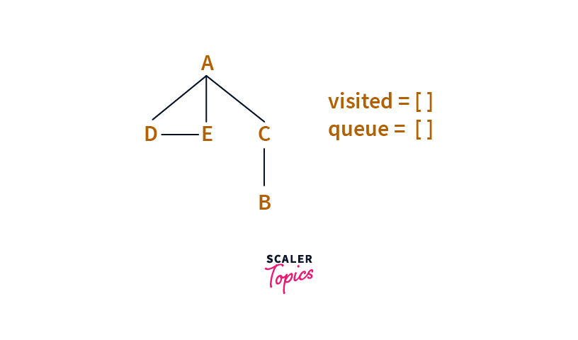
Step: 1 We pick A as the starting point and add A to the Queue. To prevent cycles, we also mark A as visited(by adding it to the visited set).

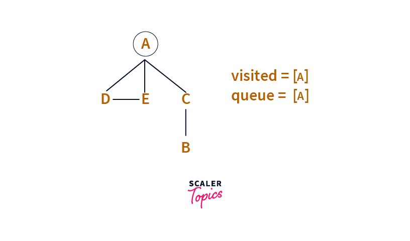
Step: 2 We remove the head of the Queue(i.e. A now). It’s the Node that was First In (inserted first) in the queue.
We process A and pick all its neighbours, which are not visited yet(i.e. not in the visited set). Those are D, C, and E.
We add D, C, and E to the Queue and also add these to the visited set.

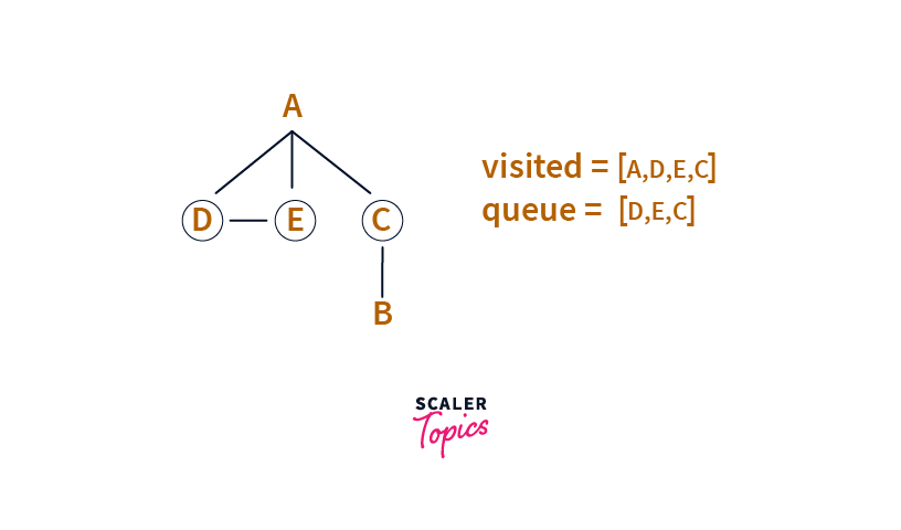
Step :3 Next, we pull the head of the Queue, i.e. D.
We process D and we consider all neighbours of D which are A and E, but since both A and E are in the visited set, we ignore them and move forward.

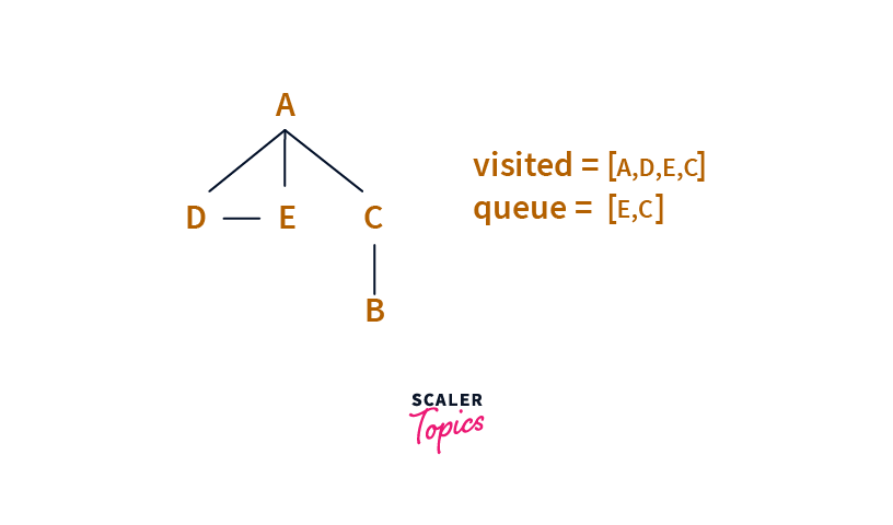
Step :4 Next, we pull the head of the Queue, i.e. E.
We process E.
Then we need to consider all neighbours of E which are A and D, but since both A and D are in the visited set, we ignore them and move forward.

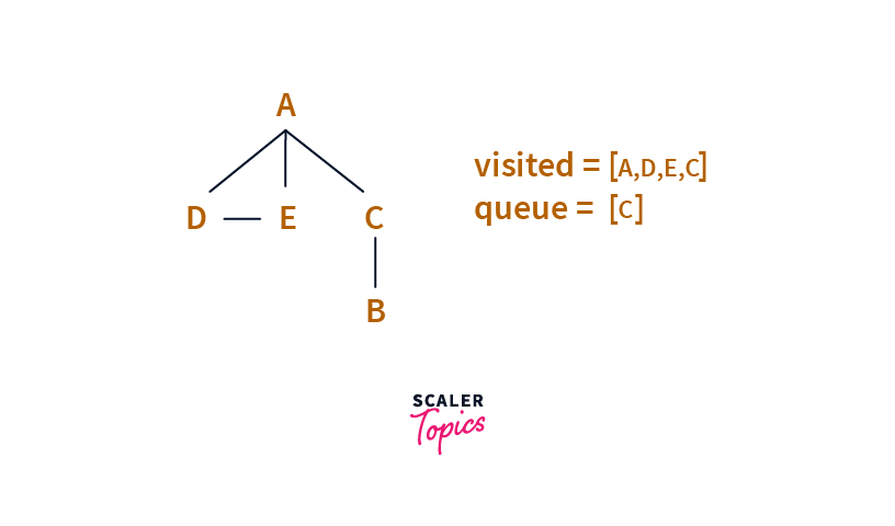
Next, we pull the head of the Queue, i.e. C.
We process C.
Then we consider all neighbours of C which are A and B. Since A is in the visited set, we ignore it. But as B is not yet visited, we visit B and add it to Queue.

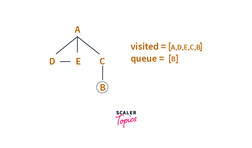
Step 5: Finally, we pick B from Queue, and its neighbour is C which is already visited, and we have nothing else in Queue to process, which means we are basically done with traversing the graph.

So the order in which we processed/explored the elements are: A, D, E, C, B which is the Breadth-First Search of the above Graph.

So we see that the Breadth-First Search relies on 2 other data structures i.e. A queue and a Visited Set (or Arrays).

Queue ensures that we process elements in the order they were first seen, and Set(or Arrays) can be used to identify which elements have already been visited before.

Pseudocode of Breadth-First Search

Rules of Breadth-First Search Algorithm

Some important rules to keep in mind for using the Breadth-First Search algorithm:

1. A Queue(which facilitates the First In First Out) is used in Breadth-First Search.
2. Since Graphs have no Root, we can start the Breadth-First Search traversal from any Vertex of the Graph.
3. While Breadth-First Search, we visit all the Nodes in the Graph.
4. For every Node already visited, we visit all of its unvisited neighbouring Nodes and add them to Queue.
5. Breadth-First Search continues until all Vertices in the graph are visited.
6. There are no loops caused in Breadth-First Search, as we prevent revisiting the same Node by marking them visited.

Implementation of Breadth-First Search Algorithm

The flow of the algorithm for Breadth First Search can be described in the following steps-

Step 1 (inside the main method): We start by creating the graph and to do that we will use an adjacency list to represent the graph. An adjacency list representation for the graph associates each vertex in the graph with the collection of its neighbouring vertices or edges.

Each vertex in the graph is associated with a list of its adjacent vertices. So, if there are edges 1---2, and 1---3 in the graph, then the List for vertex 1 will have 2 and 3 (i.e neighbours of node 1).

Similarly, List for node 2 will have 1 and List for Node 3 will have 1 too.

Please note that here we are putting 1 against 2, and 2 against 1 for an edge of 1---2. So we are forming an undirected graph.

Complexity Analysis of Breadth First Search

Time Complexity Analysis:

If we notice carefully, Breadth-First Search tries to visit one vertex at a time, until all are visited. From each vertex, we explore all of its neighbouring vertices, which is nothing but iterating all vertices connected to it on all of its edges.

So this essentially boils down to visiting each Vertex, and we have V total vertices.

From each V, we iterate all of the other neighbour vertices i.e. at the other end of all of its edges, and the total edges that we can have in the graph is E. Then it means Breadth-First Search works in O(E + V) time.

Space Complexity Analysis:

We use two data structures in Breadth-First Search - the visited array/Set, and the Queue.
A Visited array will have the size of the number of vertices in the graph (Similarly, the maximum size of a Set can also be up to the number of vertices in the graph).

Queue carries the vertices, as it explores them, and the maximum nodes it can have is again as many as the vertices in the Graph. E.g. If the starting vertex is 0 and all other vertices are connected to 0, then when we explore 0, we add all other vertices(as those are neighbours of 0) to Queue. So, the Queue will carry V-1 vertices in the worst case.

Since both the Visited array and Queue can have a max size of V(equal to as many vertices), the overall space complexity will be O(V).

Applications of Breadth First Search Algorithm

Let’s try to see where does Breadth-First Search finds its applications:

1. Minimum spanning tree for unweighted graphs- In Breadth-First Search we can reach from any given source vertex to another vertex, with the minimum number of edges, and this principle can be used to find the minimum spanning tree which is the path covering all vertices in the shortest paths.
2. Peer to peer networking: In Peer to peer networking, to find the neighbouring peer from any other peer, the Breadth-First Search is used.
3. Crawlers in search engines: Search engines need to crawl the internet. To do so, they can start from any source page, follow the links contained in that page in the Breadth-First Search manner, and therefore explore other pages.
4. GPS navigation systems: To find locations within a given radius from any source person, we can find all neighbouring locations using the Breadth-First Search, and keep on exploring until those are within the K radius.
5. Broadcasting in networks: While broadcasting from any source, we find all its neighbouring peers and continue broadcasting to them, and so on.
6. Path Finding: To find if there is a path between 2 vertices, we can take any vertex as a source, and keep on traversing until we reach the destination vertex. If we explore all vertices reachable from the source and could not find the destination vertex, then that means there is no path between these 2 vertices.
7. Finding all reachable Nodes from a given Vertex: All vertices which are reachable from a given vertex can be found using the BFS approach in any disconnected graph. The vertices which are marked as visited in the visited array after the BFS is complete contains all those reachable vertices.

See more

• Breadth First Search in Python
• BFS Program in C