Dynamic Programming
Video Tutorial
Overview
Dynamic Programming is an approach to solve problems by dividing the main complex problem int smaller parts, and then using these to build up the final solution. In layman terms, it just involves a repeating formula and some base cases. It is a technique that is mostly used in problems that can be broken down into smaller and smiliar problems whose results are stored so they can be used again.
Recursion is a prerequisite for Dynamic Programming.
Scope of Article
- This article defines Dynamic Programming and explains the intuitive logic of this technique. We also learn how it works, its characteristics, and its applications.
- The article tells about characteristics of dynamic Programming
- The article tells about components of dynamic Programming
- The article tells about elements of dynamic Programming
Takeaways
Dynamic programming can reduce the time needed to perform a recursive algorithm.
What is Dynamic Programming
Consider the famous mathematical concept of factorials. It is denoted by the symbol . And the factorial of a number is equal to the product of numbers from 1 to that number. So,
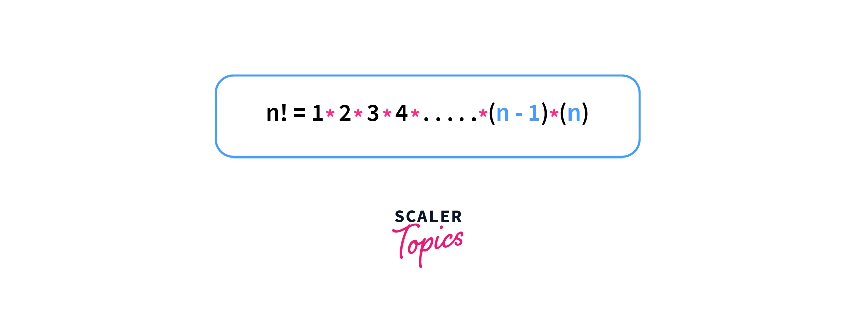
Suppose, we want to compute the factorials for all numbers from 1 to n. That means we would have to iterate from 1 to n, and for each , we will have to compute the product from 1 to i.
The above code will give us the factorial values from 1 to n. But what will be the time complexity for this code?
The outer loop runs till n, and so does the inner loop when i = n. So, overall complexity is . This is too high and expensive for values of .
So, what can we do to decrease this complexity? One thing to notice is that there is something common in and .
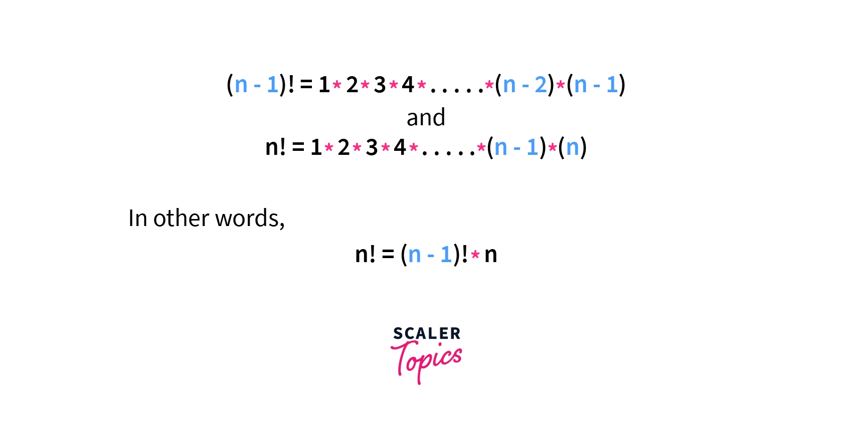
That means we can use the previously computed value of to compue , we need not iterate completely from 1 to n. So we would just need some extra space to store the previously computed values and done.
In this case the time complexity drastically reduces to , by just using some extra space.
This is exactly what Dynamic Programming is all about. We combine the previously computed solutions to get our final answer. And to speed things up, we store the solutions to these smaller problems, in case they are required again.
These problems whose solutions can contribute to the final answer are called subproblems, as they are like a smaller and similar version of the original question.
Hence, in dynamic programming, we store the solutions of subproblems. So, we break a complex problem into subproblems of similar structure, whose results are stored in memory (structures like array/map in C++ or ArrayList/HashMap in Java can be used) so that they can be retrieved efficiently and used again.
If you dont remember what you did in the past, you tend to repeat the same mistakes again and again, so the final solution can be computed much more efficiently if the values of the previous subproblems are stored as we don't have to compute them again.
In the case of any dynamic programming problem, when we divide the problem, the subproblems are not independent, instead the solutions to these subproblems are used to compute the values for the larger problems.
These repeating subproblems are used again and again and hence their results are stored. If the results of subproblems are not stored, we would have to compute them again and again, which will be very costly.
So, even if we can solve a problem with plain iteration/recursion, dynamic programming makes it faster and more efficient by using some extra space.
For example, we could work without storing the solutions to the factorials in the memory, but then we would have to recompute it again and again when computing the factorial for the next numbers. By storing these values, we can just return them quickly, thus reducing response time.
Highlights: In Dynamic Programming, complex problems are divided into smaller but similar subproblems whose results are stored and used again.
Example of Dynamic Programming
To understand Dynamic Programming more clearly, let us look at an example.
Suppose we want to reconstruct the Fibonacci Series. It is a series, which starts with 0 and 1, and each consecutive term is the sum of the previous two terms in the series.
So, the first few terms of the Fibonacci Series are: 0, 1, 1, 2, 3, 5, 8, and so on. It is very clear that to calculate each term after the first two terms, we will need the previous two terms of the series.
Let's try to solve this problem using Recursion. The nth term can be calculated by adding its previous two terms. The base cases for the recursion will be the first two terms of the series which are 0 and 1. Hence, the recursive solution would be:
A recursion tree for the Fibonacci sequence.
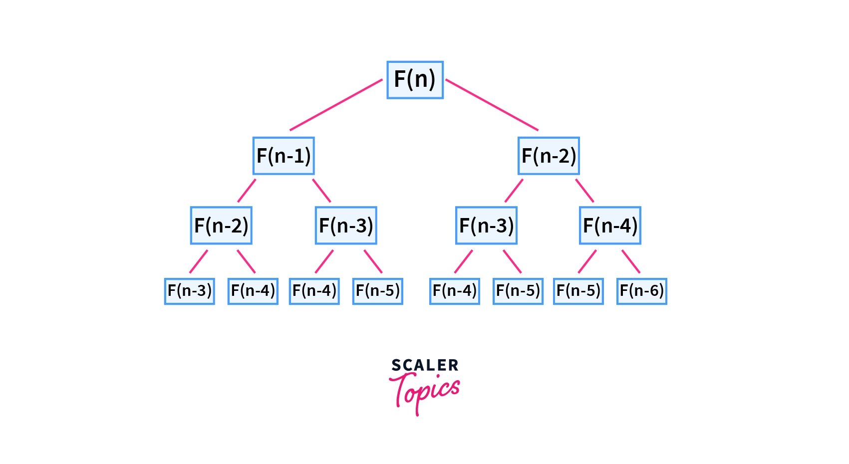
It can be easily observed from the recursion tree that a particular recursive call, say F(n-2) is being used multiple times. In a purely recursive solution, we compute it again and again, hence making the solution unnecessarily expensive in terms of time complexity.
Now if we look at the dynamic Programming approach, instead of recomputing these repeating terms again, we will just store them and use the pre-calculated values, making the solution much more efficient.
Let us look at the dynamic programming solution to find the sixth term of the Fibonacci series.
The process we will follow is:
- The (0-indexed) fifth term, F[5] = F[4] + F[3]. We recurse for F[4] and F[3].
- The (0-indexed) fourth term, F[4] = F[3] + F[2]. We recurse for F[3] and F[2].
- The (0-indexed) third term, F[3] = F[2] + F[1]. We recurse for F[2] and F[1].
- The (0-indexed) second term, F[2] = F[1] + F[0]. We recurse for F[1] and F[0].
- The zero-th and first terms are base cases of a Fibonacci Series. So, F[0] = 0 and F[1] = 1. These are stored in memory to be used again.
- From here we return to calculating our second term, F[2] = F[1] + F[0] = 1 + 0 = 1. Note, that the already computed and stored values of F[0] and F[1] are used. Again, this is stored.
- We return to calculating our third term, F[3] = F[2] + F[1] = 1 + 1 = 2. Note, that the already computed and stored values of F[2] and F[1] are used. F[3] is stored in memory.
- We return to calculating our fourth term, F[4] = F[3] + F[2] = 1 + 2 = 3. Note, that the already computed and stored values of F[3] and F[2] are used. F[4] is stored in memory.
- We return to calculating our fifth term, F[5] = F[4] + F[3] = 2 + 3 = 5. Note, that the already computed and stored values of F[4] and F[3] are used. F[5] is stored in memory.
- We have avoided a lot of recomputation by storing the solutions to subproblems.
F[5] = F[3] + F[4]
F[4] = F[2] + F[3]
F[3] = F[1] + F[2]
F[2] = F[0] + F[1]
F[1] = 1 (Base Case)
F[0] = 0 (Base Case)
F[2] = F[0] + F[1] = 0 + 1 = 1
F[3] = F[1] + F[2] = 1 + 1 = 2
F[4] = F[2] + F[3] = 1 + 2 = 3
F[5] = F[3] + F[4] = 2 + 3 = 5
If we were not using dynamic programming, we would be calculating two previous terms in each step, but because we have those values already stored, we can just use them, drastically decreasing the time complexity. To be precise, the recursive solution has exponential time complexity as we are executing two recursive calls each time until we reach the base case.
But, the dynamic programming approach has (n is the term to be calculated) or linear time complexity as we do not return to a particular term again after it has been computed once. Instead we use it's already computed and stored value if needed again. So, each term is traversed only once improving the time complexity from exponential to linear.
How Dynamic Programming Works?
Like we saw in the example of factorials, storing the solution to previous factorials in extra memory space was beneficial in reducing the overall response time. This is utilised by Dynamic Programming, which is why it is so efficient.
By storing the solutions of sub-problems in extra memory space, we thereby reduce the time taken to calculate the complete solution for a problem. This method of storing the answers to similar subproblems is called memoization.
Because of this, dynamic programming can solve a vast variety of problems involving optimal solutions, which means finding the best case out of all. In these cases also, dynamic programming takes help of smaller subproblems to reach to the final optimal solution.
In Dynamic Programming, we analyze all subproblems to find out the most optimal solution, but because we store these values, no subproblem is recomputed. This increases the efficiency of a Dynamic Programming solution and also assures a correct solution as we are basically checking all the cases, but efficienlty.
Dynamic Programming algorithm works by computing the answer to all possible subproblems and stores them to find the final answer. This process of storing values of subproblems is called memoization which helps in reaching the final solution efficiently.
Characteristics of Dynamic Programming
Two very important characteristics essential for a Dynamic Programming approach to work are:
- Optimal Substructure
- Overlapping Subproblems
To understand things more clearly, let us take example. Suppose there is a flight of n stairs. You are at the bottom and want to reach the top stair. Climbing the ith stair costs cost[i]. At each stair you have an option of either moving to the (i+1) th stair, or skipping one stair and jumping to the (i+2) th stair. We need to find the minimum cost to climb the topmost stair.
In the end we need to find the minimum cost possible, that means this problem involves making optimal choices, that is finding the best option. Looking closely, we can see that if we break the problem such that we first find the minimum cost to reach the first stair, then the minimum cost to reach the second stair and so on, the end solution will be easily computable.
For example, suppose we have 5 stairs with cost of climbing each step given by the array cost:
cost[] = [2,5,10,4,1]
We are below the bottom most stair. We divide this problem into smaller problems as : What will be the minimum cost to reach the ith stair. We also store these solutions to the subproblems in the ans[] array, as they will be needed again.
The base cases will be when i = 0, that means when there is no stair to climb and when i = 1.
For i = 0, we don't need to climb any stairs so
ans[0] = 0
When i = 1, we want to find the minimum cost to climb the first stair. This will be our base case, as there is only one way to reach the first stair, which is to climb it. So,
ans[1] = cost[1] = 2.
For i = 2, we have two cases to choose from. We can either climb to the second stair directly from below the stairs, or by climbing one step from the first stair.Here we have a choice, and as we need to minimise the total cost, we will choose the one which gives us minimum cost.
ans[2] = min(cost[2]+ans[0],cost[2]+ans[1])
Here, cost[2] is the cost to climb to the second step directly from the bottom and cost[2]+ans[1] is the total cost to climb to the second step by climbing first step in between.
Now, if we hadn't stored the solution for the first step in ans[1], we would have to compute it again.
By making these optimal choices at smaller steps, we will be able to compute the overall optimal solution. This is what is meant by Optimal Substructure.
For i = 3, we again have two cases to choose from. We can either climb to the third stair by jumping directly from the first stair, or by climbing one step from the second stair. Again, we have a choice, and as we need to minimise the total cost, we will choose the one which gives us minimum cost.
ans[3] = min(cost[3]+ans[1],cost[3]+ans[2])
Here, cost[3] + ans[1] is the cost to climb to the third step by jumping from the first stair and cost[3] + ans[2] is the total cost to climb to the third step by climbing climbing one step from the second stair.
Again, if we hadn't stored the solutions for the first and second stair in the answer array, we would be recomputing it, and this would be the second round of recomputation.
This means that the same smaller subproblem is needed to be computed again and again. Also, these subproblems, differ only in their parameters which is the value of the stair, but the optimal choice we need to make at each step remains the same. This is what is meant by Overlapping Subproblems.
In general, the answer for the nth stair will be
ans[n] = min(cost[n]+a ns[n-1],cost[n]+ans[n-2])
ans[n-1] will be the minimum cost to reach to the (n-1)th stair while ans[n-2] is the minimum cost to reach the (n-2)th stair. This can be rewritten as
ans[n] = cost[n] + min(ans[n-1],ans[n-2])
as cost[n] is common to both, as we will have to pay cost[n] to climb to the nth stair.
As this climbing stairs problem satisfies both the Optimal Substructure as well as the Overlapping Subproblems property, hence it can be solved by using a dynamic programming approach.
Now let's define both of these in detail.
Optimal Substructure
If a complex problem has an Optimal Substructure property it means that to find an optimal solution for the problem, the optimal solutions of its smaller subproblems are needed.
So, by combining the optimal solutions of subproblems, we can obtain a solution efficiently.
This property is used by the Dynamic Programming algorithm to ensure a correct solution to the given problem.
Taking the example of the Fibonacci Sequence again, the nth term is given by :
F(n) = F(n-1) + F(n-2)
So, to find the nth term, we need to find the correct solution for the (n-1)th and the (n-2)th term, which are smaller subproblems of the complete problem. And again to find the (n-1)th term and the (n-2)th term, we need to find the solution to even smaller subproblems.
Overlapping Subproblems
A problem is said to have Overlapping Subproblems property if it can be broken down into smaller parts called subproblems, which need to be solved again and again. This means that the same subproblem is needed again and again to generate the final solution.
This property is used by Dynamic Programming in the sense that it stores the solutions to these recurring subproblems so that we do not need to compute it again and again.
For example, in the Fibonacci Sequence problem, we have
F(n) = F(n-1) + F(n-2)
F(n-1) = F(n-2) + F(n-3)
F(n-2) = F(n-3) + F(n-4)
F(n-3) = F(n-4) + F(n-5)
From this, it is clear that the subproblems F(n-2), F(n-3), and F(n-4) are used again and again to find the final solution.
Components of Dynamic Programming
The major components in any Dynamic Programming solution are:
- Stages
- States and state variables
- State Transition
- Optimal Choice
We now know how Dynamic Programming works, but how do we start building a Dynamic Programming solution? The major components needed to construct a Dynamic Programming solution are discussed below.
Stages
When a complex problem is divided into several subproblems, each subproblem forms a stage of the solution. After calculating the solution for each stage and choosing the best ones we get to the final optimized solution.
For example, in the previous instance of the climbing stairs problem, we needed the minimum cost to reach the (i-1) th and the (i-2) th stair first. That means to find ans[n], we had to calculate the values of ans[n-1] and ans[n-2] first. Hence, here ans[n-1] and ans[n-2] are different stages whose solution we need to find to get to the value of ans[n] finally.
States and State Variables
Each subproblem can be associated with several states. States differ in their solutions because of different choices. A state for a subproblem is therefore defined more clearly based on a parameter, which is called the state variable. It is possible in some problems, that one than one variable is needed to define a state distinctly. In these cases, there are more than one state variables.
For example, we could reach the nth stair by either jumping up from the (n-2)th stair or by climbing one step from the (n-1)th stair. Hence, these are the two states related to reaching the nth stair in minimum cost and the variable which is the stair number from which we are climbing up to the current stair, is the state variable that defines a state uniquely.
State Transition
State Transition simply refers to how one subproblem relates to other subproblems. By using this state transition, we calculate our end solution.
For example, in the climbing stairs problem, the state transition was:
ans[n] = cost[n] + min(ans[n-1],ans[n-2])
Here ans[n] represents the minimum cost to reach the nth stair.
Using this state transition, we can know how different subproblems relate to each other, which can be used to compute the final optimal solution.
Optimal Choice
At each stage, we need to choose the option which leads to the most desirable solution. Choosing the most desirable option at every stage will eventually lead to an optimal solution in the end.
For example, in the climbing stairs problem, we need to make an optimal choice based on whether we get a minimum cost by clmbing from the stair directly beneath the current one, or by jumping from two stairs below. We need to make this optimal choice at each stair, to reach to the final solution at the end.
Elements Of Dynamic Programming
Three elements of the Dynamic Programming algorithm are :
- Substructure
- Table Structure
- Bottom-Up Computation
The elements in a Dynamic Programming Solution are discussed below:
- To solve a given complex problem and to find its optimal solution, it is broken down into similar but smaller and easily computable problems called subproblems. Hence, the complete solution depends on many smaller problems and their solutions. We get to the final optimal solution after going through all subproblems and selecting the most optimal ones. This is the substructure element of any Dynamic Programming solution.
- Any Dynamic Programming solution involves storing the optimal solutions of the subproblems so that they don't have to be computed again and again. To store these solutions a table structure is needed. So, for example arrays in C++ or ArrayList in Java can be used. By using this structured table, the solutions of previous subproblems are reused.
- The solutions to subproblems need to be computed first to be reused again. This is called Bottom-Up Computation because we start storing values from the bottom and then consequently upwards. The solutions to the smaller subproblems are combined to get the final solution to the original problem.
Approaches to Dynamic Programming
There are two types of approach that can be used to solve a problem by Dynamic Programming:
- Memoization or Top-Down Dynamic Programming
- Tabulation or Bottom Up Dynamic Programming
We've seen the working and characteristics of Dynamic Programming. But how are the solutions to subproblems exactly stored?
For this, two major approaches can be used while solving a problem by a Dynamic Programming approach. These are:
- Memoization or Top-Down Approach (Recursion is used in this approach)
- Tabulation or Bottom-Up Approach (Here we use iterative approach i.e for loops)
Top Down Dynamic Programming
As the name suggests, to find out the solution to a problem we start from the top, moving down to smaller subproblems according to the state transition.
This means that we start from the most complex problem, then we try to find out the subproblems that need to be computed to solve this problem and solve them. These subproblems can be directly identified if we know the state transition of the problem.
So, in this fashion, we keep moving downwards until we reach the base cases. For example, in the Fibonacci series, the base case is for the first and second term, which will be 0 and 1 respectively.
On the way, we keep storing the values of all the subproblems which are computed so they can be reused. This process of storing the values of subproblems is called Memoization. It must be clear that the solutions to only those subproblems are calculated which are needed to compute the final solution.
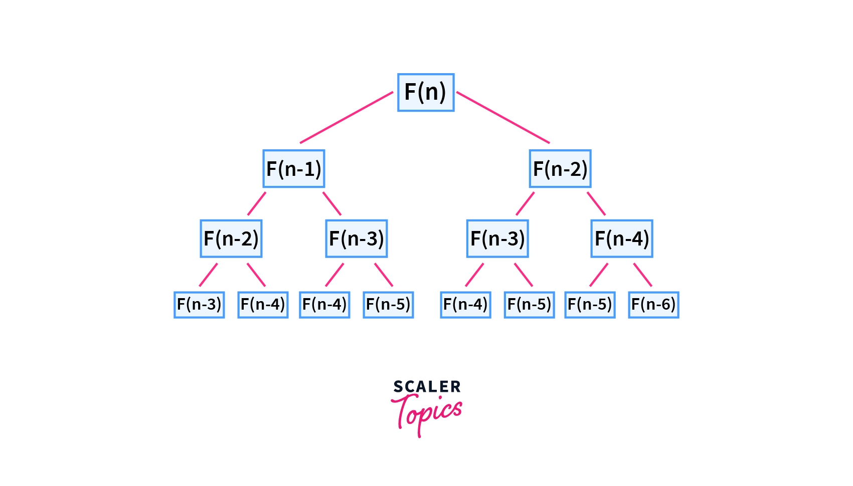
If we try to solve the Fibonacci Series problem by using the Top-Down Dynamic Programming approach, we would start by computing the value for F[n]. From the state transition, we know for this we need to have the solution to both F[n-1] and F[n-2]. So, we compute those, again for that we will have to compute F[n-3] and F[n-4].
The process goes on until we reach the base cases of F[0] and F[1] from where the solutions to all subproblems are computed and subsequently, we get the answer F[n]. On the way, we keep memoizing our solutions, and they are reused.
Bottom Up Dynamic Programming
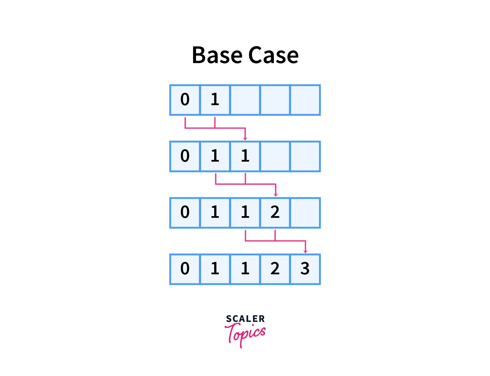
As the name suggests, to find out the solution to a problem we start from the base cases, moving up towards more complex and larger subproblems until we reach the solution we need to find. This is done by following the state transition.
This means that we start from the base cases and then sequentially go on computing the larger subproblems by using the solutions of the already solved smaller subproblems following the state transition.
So, in this fashion, we keep moving upwards until we reach the desired state. On the way, we keep storing the values of all the subproblems in a table sequentially. If needed, these values are accessed directly from the table.
This process of storing the values of subproblems is called Tabulation. It must be clear that the solutions to all subproblems are calculated, whether it contributes to the overall solution or not.
If we try to solve the Fibonacci Series problem by using the Bottom Up Dynamic Programming approach, we would start with initializing the base cases in the table as F[0] = 0 and F[1] = 1. Then we move on to compute F[2]. From the state transition, we calculate F[2] = F[1] + F[0], which have already been initialized and are accessed from the table. The process goes on until we reach the desired state. On the way, we keep tabulating our solutions, and they are reused.
Applications Of Dynamic Programming
The various applications of Dynamic Programming are :
- Longest Common Subsequence
- Finding Shortest Path
- Finding Maximum Profit with other Fixed Constraints
- Job Scheduling in Processor
- BioInformatics
- Optimal search solutions
Summary
- Dynamic Programming solves optimization problems by dividing them into smaller but similar subproblems whose results are stored and used again.
- Dynamic Programming algorithm works by computing the answer to all possible subproblems and storing them to find an optimal answer. This process of storing values of subproblems is called memoization.
- A problem can be solved by using the Dynamic Programming algorithm if it follows these two characteristics:
- Optimal Substructure
- Overlapping Subproblems
- The major components in any Dynamic Programming solution are:
- Stages
- States and state variables
- State Transition
- Optimal Choice
- Three elements of the Dynamic Programming algorithm are :
- Substructure
- Table Structure
- Bottom-Up Computation
- here are two types of approaches that can be used to solve a problem by Dynamic Programming :
- Memoization or Top-Down Dynamic Programming
- Tabulation or Bottom Up Dynamic Programming
- Dynamic Programming finds its applications in different areas like BioInformatics, finding the shortest path, and many more.
