RMSProp

Overview

RMSProp, which stands for Root Mean Squared Propagation, adapts the gradient Descent Algorithm for Optimization. It comes under the category of adaptive optimization Algorithms. These adaptive Optimizers have resulted in faster and more efficient learning time. We will look into RMSProp by first looking at RProp, understanding its defects, and then learning how RMSProp solves them.

Scope

In this article, we will see what adaptive optimizers are and why we need them.
We'll look into the advantages RMSProp has over Rprop.
The working mechanism of RMSProp will be discussed.
We'll implement Gradient Descent using RMSProp from scratch.
Visualizing RMSProp in action.

Introduction

Root Mean Squared Propagation

Geoffrey Hinton, the father of the Backpropagation algorithm, first proposed RMSProp. RMSProp works by varying the step size at each iteration to give better results. It dampens the oscillations and reaches the minima much quicker. It uses a decaying moving average of gradients to forget the earlier gradients while prioritizing the more recent gradients in its computations.

Rprop to RMSprop

RProp, or Resilient Propagation, was introduced to tackle the problem of the varying magnitude of gradients. It introduces adaptive learning rates to combat the problem by looking at the two previous gradient signs. RProp works by comparing the sign of the previous and current gradient and adjusting the learning rate, respectively. The following Pseudo code will give a better understanding.

w[t] -> weights

dw -> Gradients wrt weights

If the previous and current gradients have the same sign, the learning rate is accelerated(multiplied by an increment factor)—usually, a number between 1 and 2. If the signs differ, the learning rate is decelerated by a decrement factor, usually 0.5.

The problem with RProp is that it cannot be implemented well for mini-batches as it doesn't align with the core idea of mini-batch gradient descent. When the learning rate is low enough, it uses the average of the gradients in successive mini-batches. This doesn't get applied in RProp. For example, if there are 9 +ve gradients with magnitude +0.1 and the 10th gradient is -0.9, ideally, we would want the gradients to be averaged and cancel each other out. But in RProp, the gradients get incremented 9 times and decremented once, which nets a gradient of a much higher value.

So ideally, we would want a technique with a moving average filter to overcome the problem of RProp while still maintaining the robustness and efficient nature of RProp. This leads us to RMSProp.

Root Mean Squared Propagation (RMSProp)

Root Mean Squared Propagation reduces the oscillations by using a moving average of the squared gradients divided by the square root of the moving average of the gradients.

V_{dw} = \beta V_{dw} + (1-\beta)dw^2

W = W - \alpha \cdot \frac{dw}{\sqrt{V_{dw}}}

The above equation is used for RMSProp. In the first equation, Vdw calculated the stepsize using the average. The variable Vdw contains the information of the previous gradients acting as a moving average. The parameter $\beta$ controls the number of previous parameters that must be considered in the first term. For most practical applications $\beta$ = 0.9.The value 0.9 means that roughly the previous 10 terms are considered. In the second term, the oscillations are reduced by considering the square of the current gradient. Intuitively, since the value Vdw is divided in the learning rate term, if Vdw is low, the learning rate increases and vice versa. So if the gradient is high, this technique smoothens it out, thus reducing the oscillations.

Gradient Descent With RMSProp

Gradient Descent is an optimization algorithm used to train Machine Learning models. It iteratively checks the gradients to find the minima of the cost function. RMSProp is an improved form of gradient Descent that uses a decaying moving average instead of just the current values.

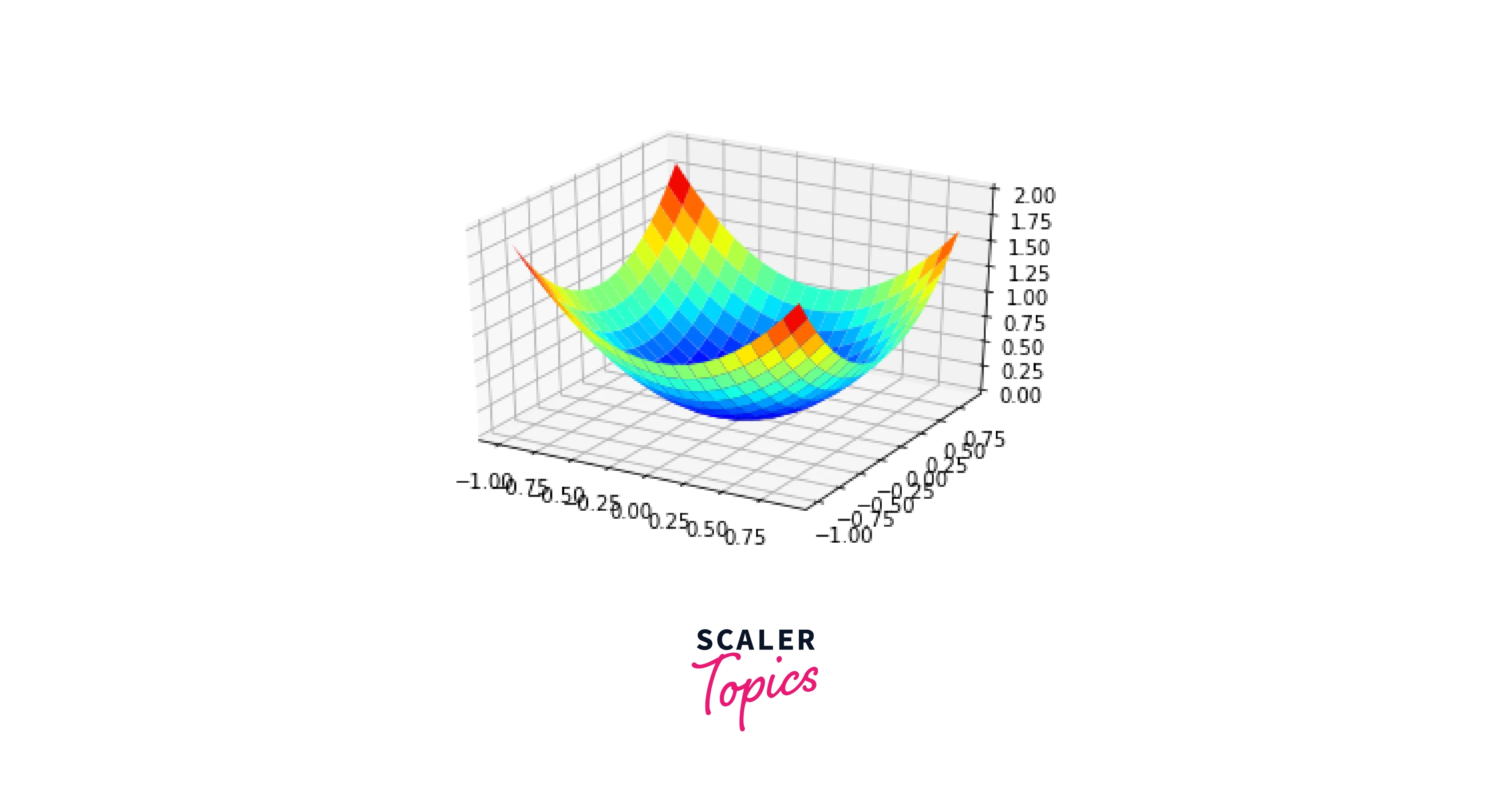
Two-Dimensional Test Problem

We're going to choose an objective test function.

objective function = $x^2$ + $y^2$

For simplicity, we will choose the bounds of our example between -1 and +1.

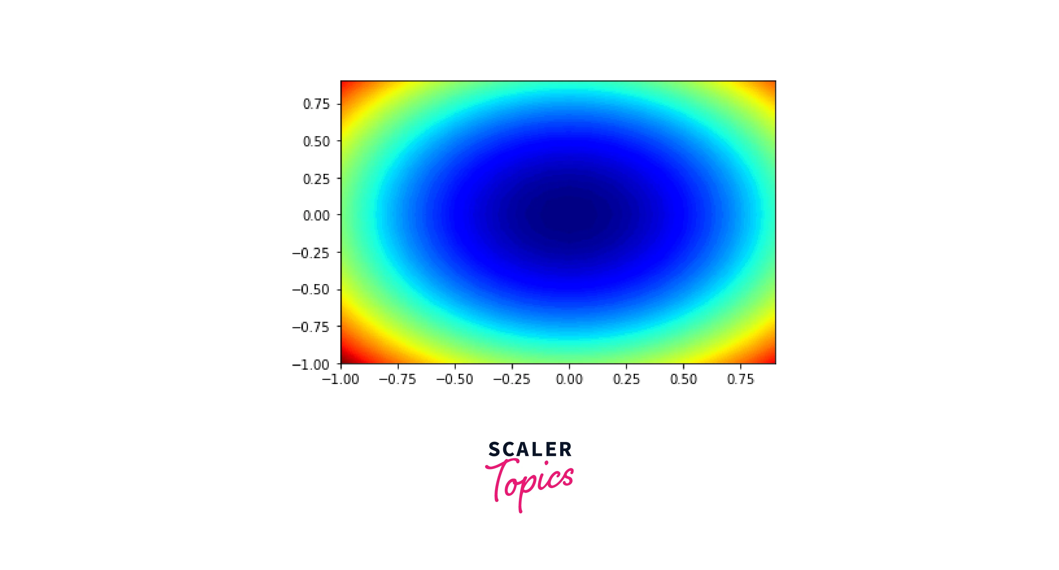
The sample rate is chosen as 0.1, and the obtained values are plotted in a 3d model and as a contour plot.

test sample 3d plot

test sample contour plot

Gradient Descent Optimization With RMSProp

First, we implement the same objective function as before, along with a gradient function. The derivative of $x^2$ + $y^2$ is $2x + 2y$

Next, we define the RMSProp model. But first, we initialize the starting point and the squared average.

We create a for loop to define the number of iterations. Then, we calculate the gradients and create another for loop to calculate the squared gradient average of each variable.

Another loop is created to update each variable's learning rate(alpha), and the corresponding weights are updated.

We append the solutions to a list, and after the iterations are complete, print out the results and return the solution.

We initialize the random seed, Bounds, beta, and step size. Then, these values are passed to the RMSProp model.

The following results are obtained.

Output:

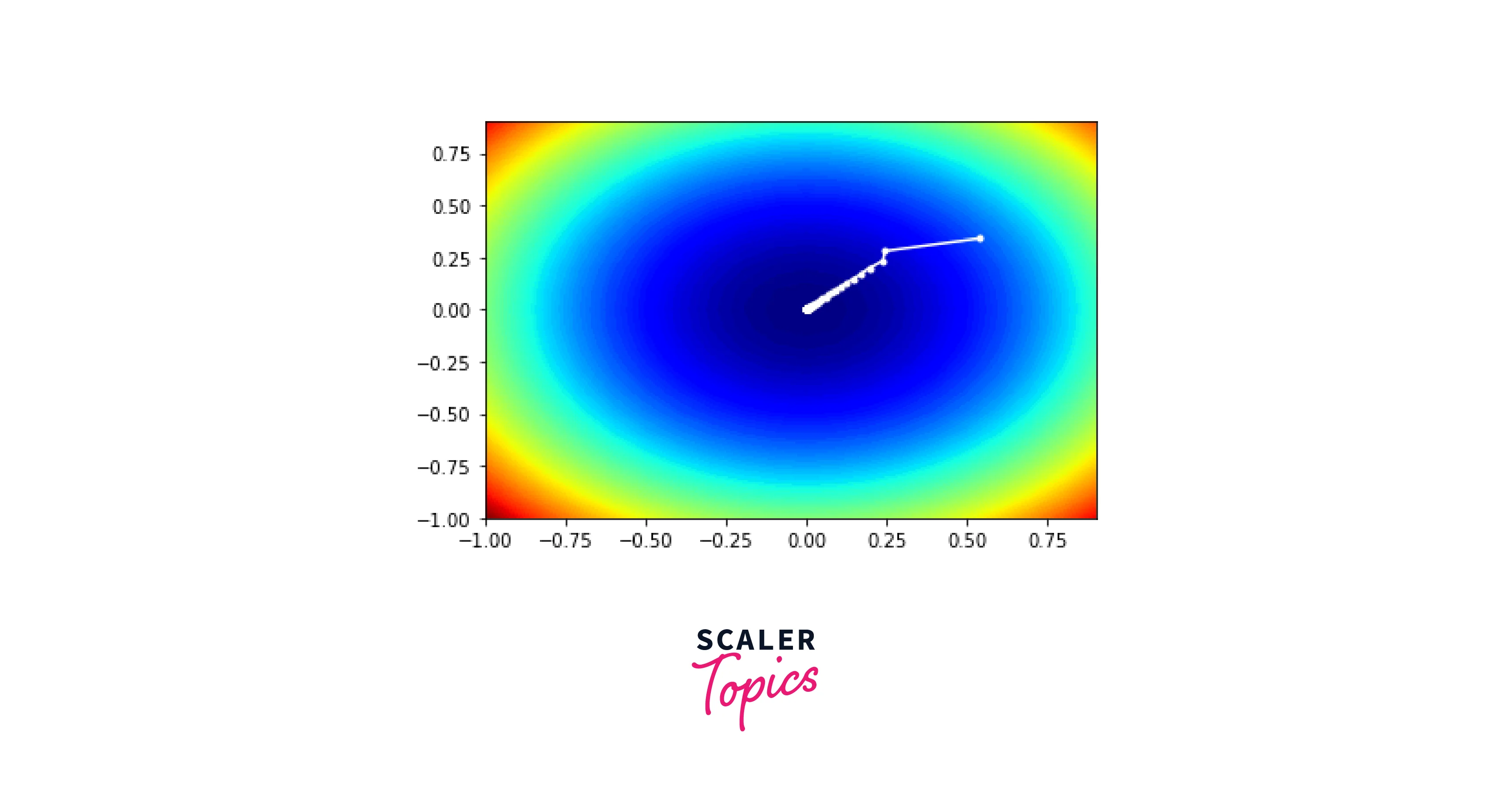
In our case, we can see that the 35th iteration reaches the minima.

Visualization of RMSProp

We use a contour plot similar to the one in the test sample. This time we add another plot within the contour plot to map the trace of solutions with each iteration. The list with all the solutions is used to plot the trace.

It gives the following plot as a result.

plot with learning trace

The entire code for RMSProp is given below.

Conclusion:

RMSProp is an adaptive learning rate optimization algorithm.
RMSProp dampens the oscillations, leading to the minimum value much quicker.
RMSprop acts as a moving average filter that considers previous gradients into account while updating the learning rate
RMSprop solves the problem of RProp's inability to work for mini-batches.

Learn via video courses