Graph Data Structure - Scaler Topics

Overview

Before actually getting started with our main agenda for this article - Graph in Data Structure, let me ask you a few questions --

Do you use social media, like facebook, twitter etc.?
Have you ever used Google Maps?
Have you used MakeMyTrip or any flight booking app?

If your answer is yes, for any of these questions, then you have already used the apps which uses graph data structure for their internal implementations and functionalities.

So, with this you must have understood how powerful graphs are. A graph is a common data structure that consists of a finite set of nodes (or vertices) and a set of edges connecting them. Graph in Data Structure have innumerable usage in real life and are used to solve real life problems.

Takeaway

A graph data structure consists of information stored in a collection of interconnected nodes(vertices) and edges(paths).

What is Graph in Data Structure?

A Graph in Data Structure is a non-linear data structure that consists of nodes and edges which connects them.

A Graph in Data Structure is a collection of nodes that consists of data and are connected to other nodes of the graph.

What is Graph in Data Structure

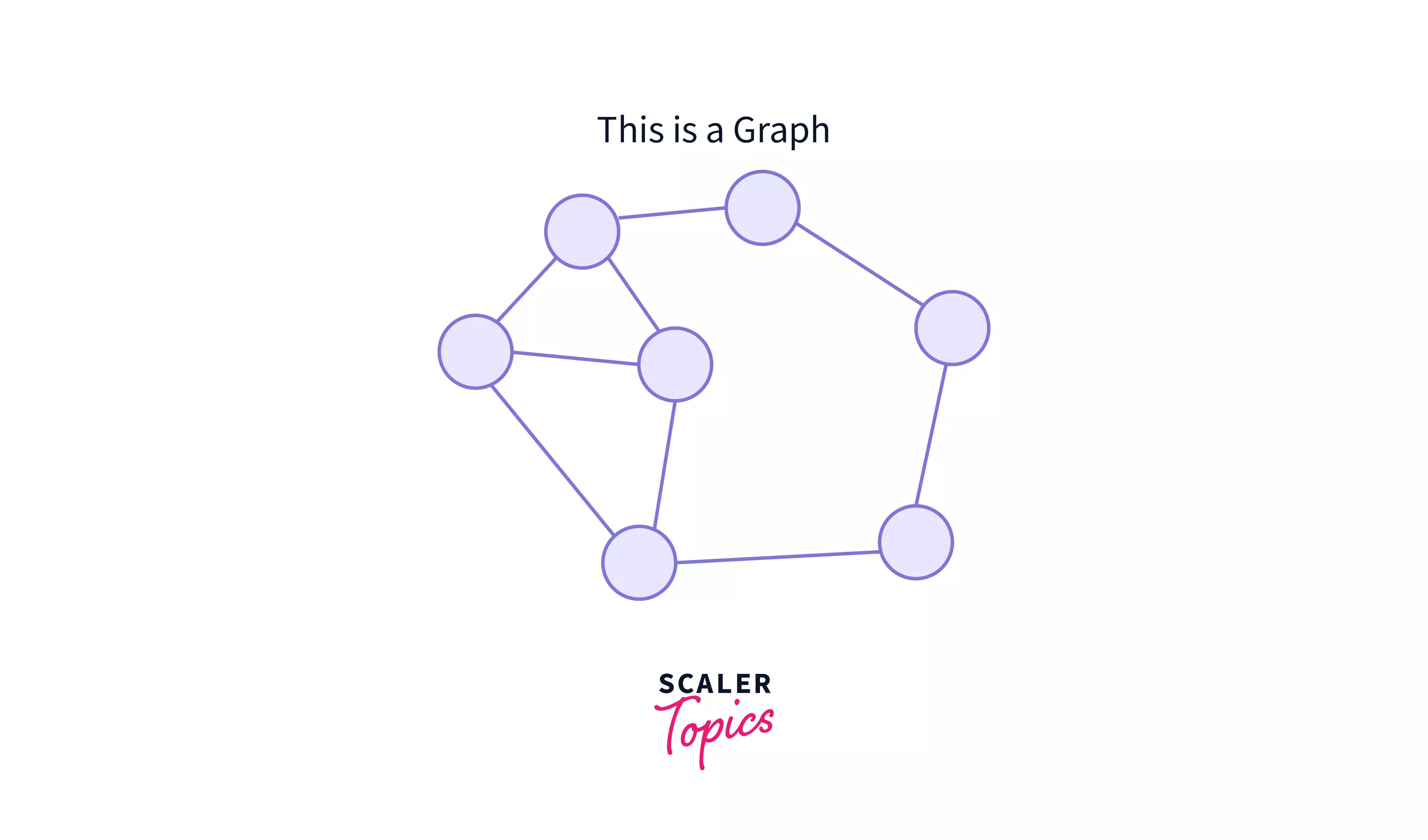
Let us now break this down into components, and understand them all --

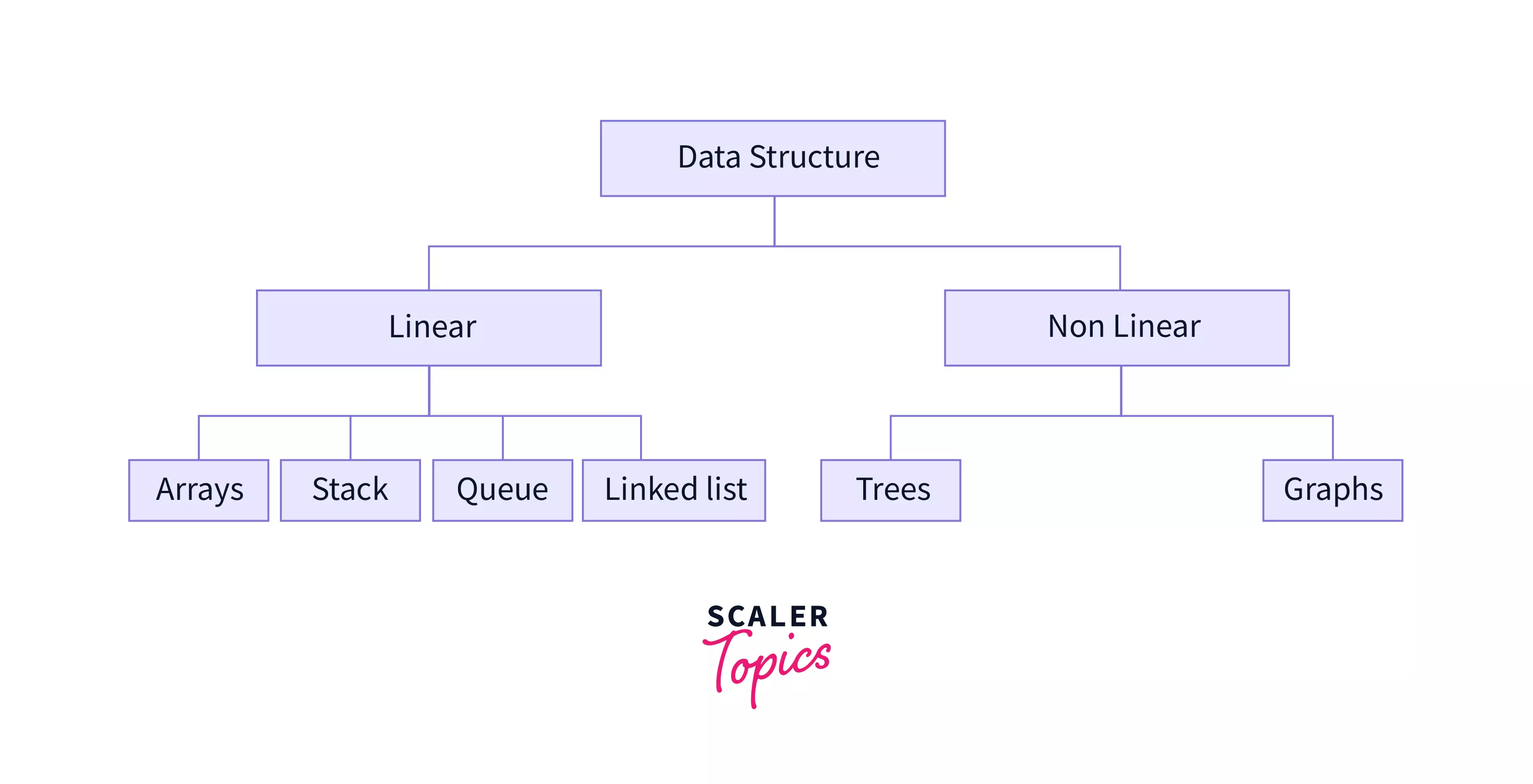
1. Non-linear Data Structure:

In a non-linear data structure, elements are not arranged linearly or sequentially. Because the non-linear data structure does not involve a single level, an user cannot traverse all of its elements at once.

2. Nodes:

Nodes create complete network in any graph. They are one of the building blocks of a Graph in Data Structure. They connect the edges and create the main network of a graph. They are also called vertices. A node can represent anything such as any location, port, houses, buildings, landmarks, etc.

They basically are anything that you can represent to be connected to other similar things, and you can establish a relation between the them.

Nodes in a graph

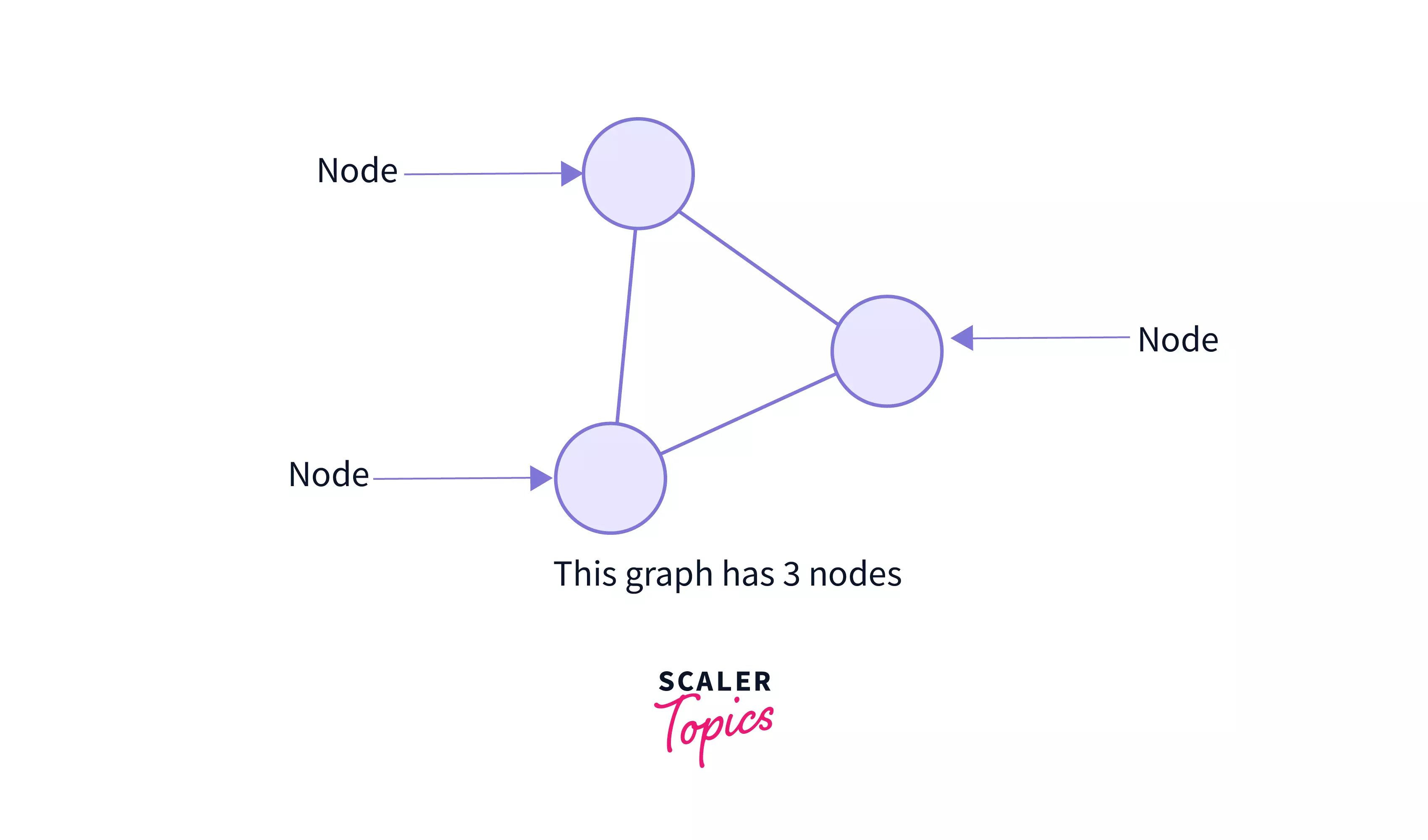
The above image represents the nodes in a graph.

3. Edges:

Edges basically connects the nodes in a Graph in Data Structure. They represent the relationships between various nodes in a graph. Edges are also called the path in a graph. Edges in a graph

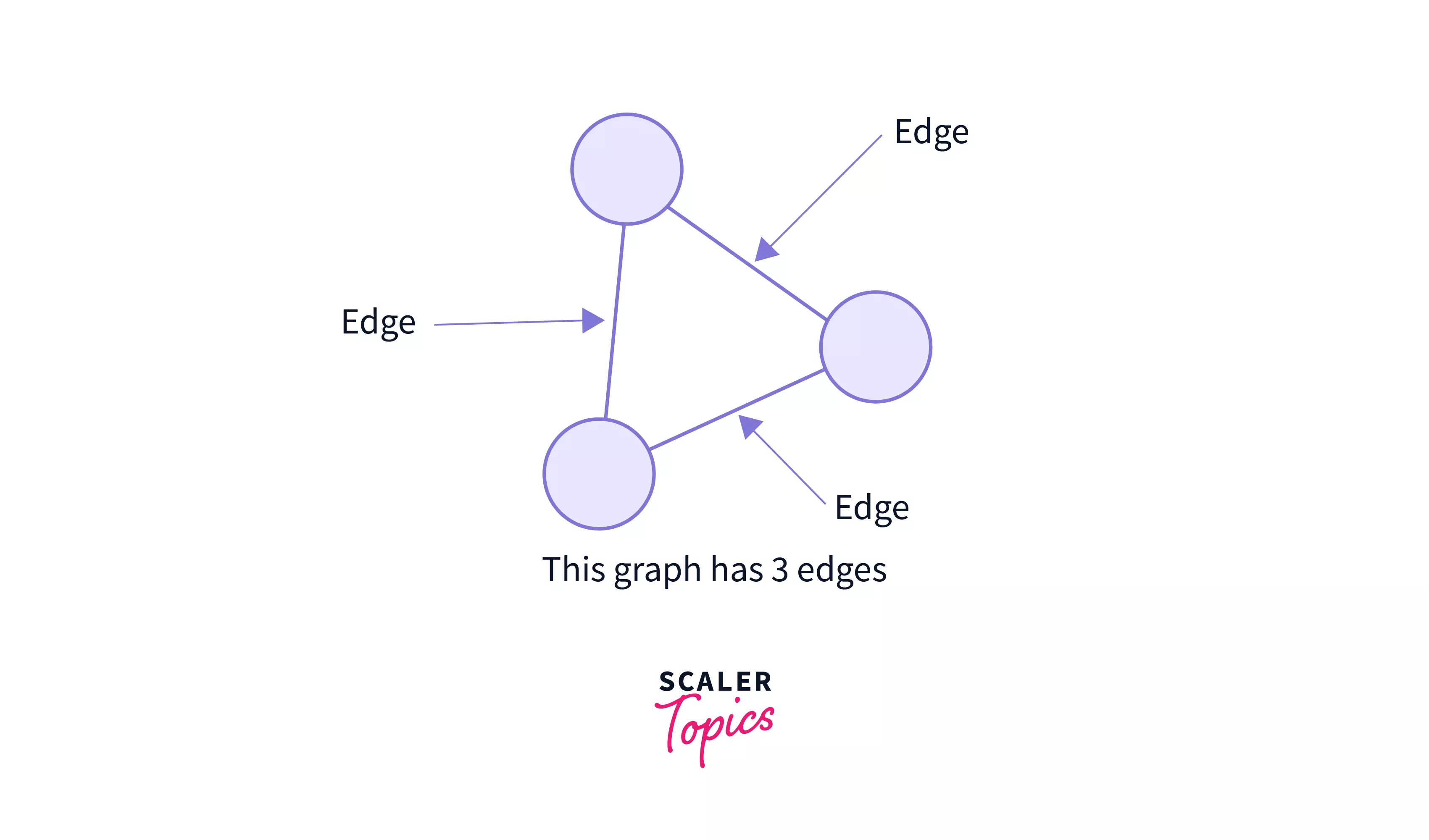
The above image represents edges in a graph.

A graph data structure $(V, E)$ consists of:

A collection of vertices $(V)$ or nodes.
A collection of edges $(E)$ or path

Example:

The below image represents a set of edges and vertices:

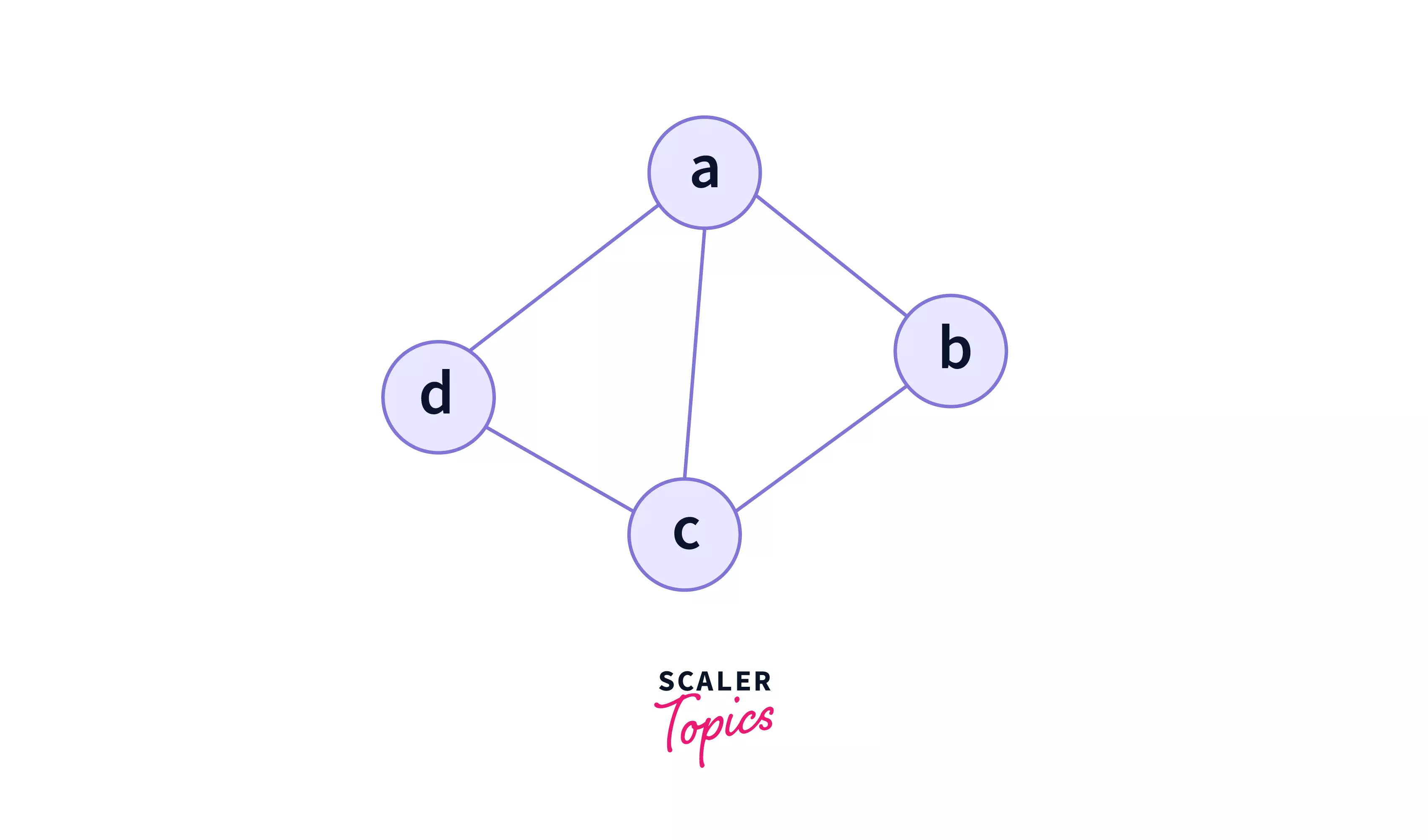
A graph is a pair of sets (V, E), where V is the set of vertices and E is the set of edges, connecting the pairs of vertices. In the above graph:

In the above graph, |V| = 4 because there are four nodes (vertices) and, |E| = 5 because there are five edges (lines).

Graph Terminology

Let us now see various terminologies associated with a graph data structure --

1. Path

A path in a graph is a finite or infinite set of edges which joins a set of vertices. It can connect to 2 or more nodes. Also, if the path connects all the nodes of a graph in Data Structure, then it is a connected graph, otherwise it is called a disconnected graph.

There may or may not be path to each and every node of graph. In case, there is no path to any node, then that node becomes an isolated node.

path in graph

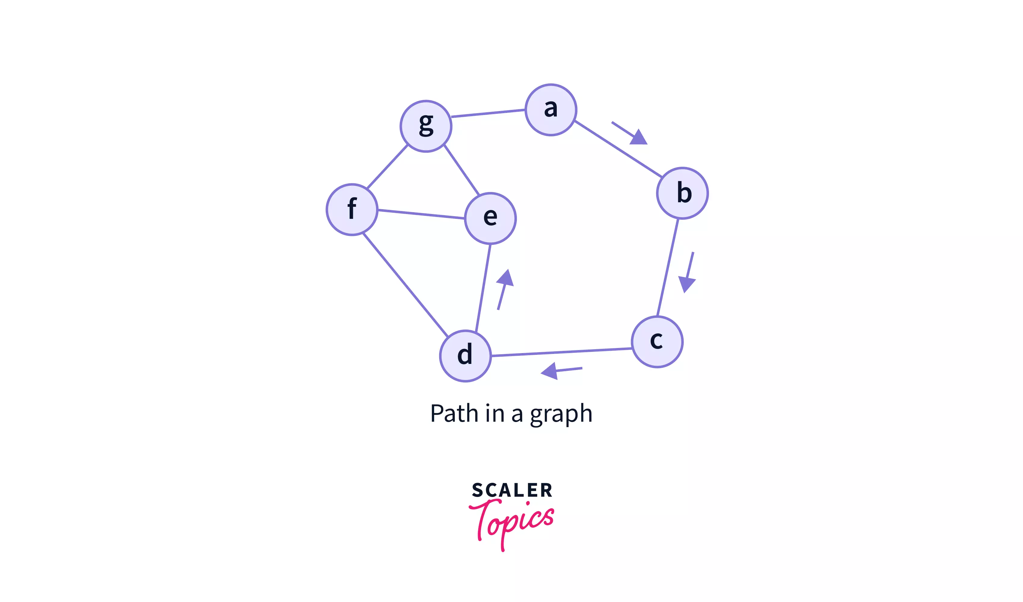
In the above graph, the path from 'a' to 'e' is = {a,b,c,d,e}

2. Closed Path:

A path is called as closed path if the initial node is same as terminal(end) node. A path will be closed path if : $V_0$ = $V_n$ , where $V_0$ is the starting node if the graph and $V_n$ is the last node. So, the starting and the terminal nodes are same in a closed graph.

Closed Path in a graph

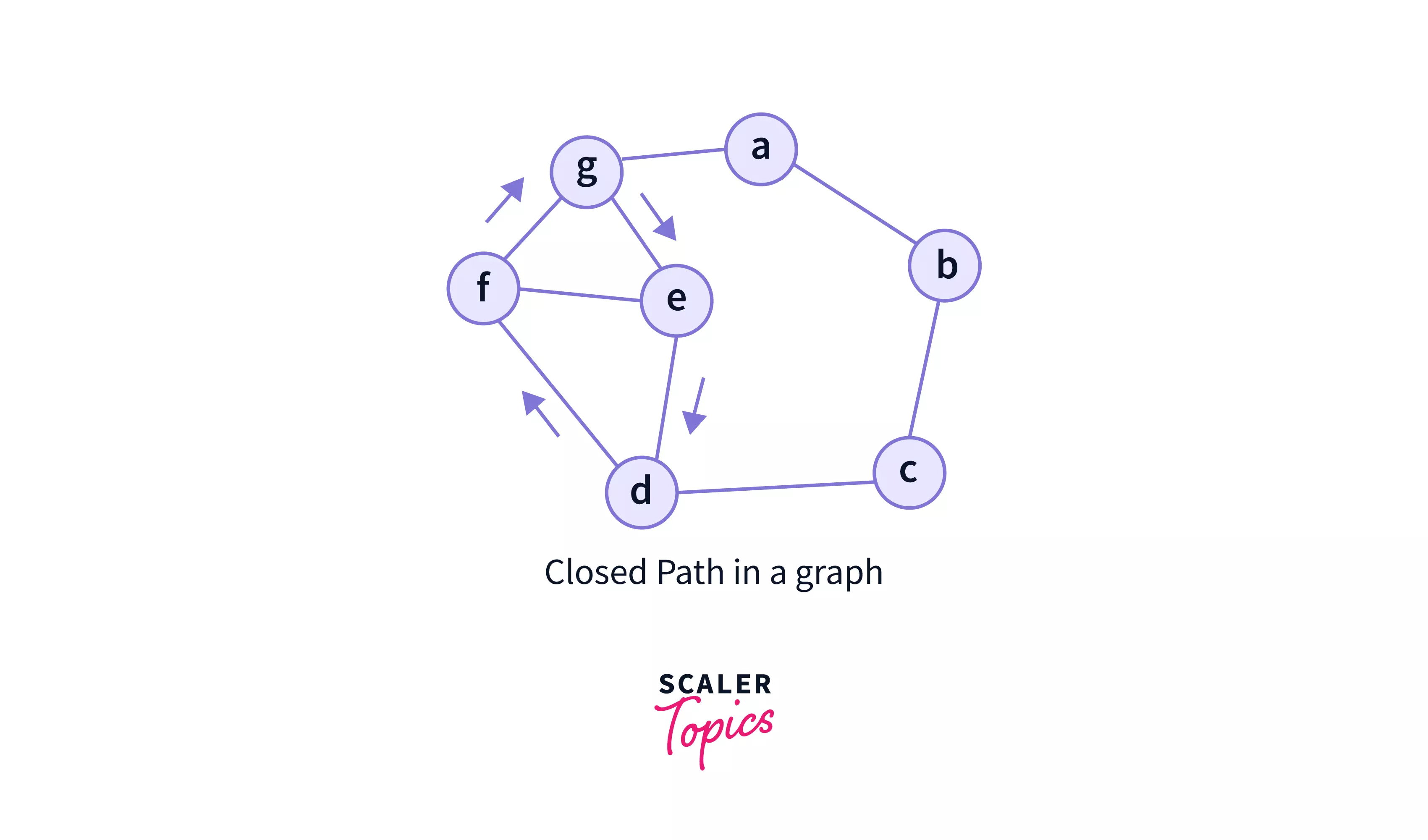
The above graph have a closed path, where the initial node = {e} is same as the final node = {e}. So, the path becomes = {e,d,f,g,e}.

3. Simple Path

A path that does not repeat any nodes(vertices) is called a simple path. A simple path in a graph exists if all the nodes of the graph are distinct, expect for the first and the last vertex, i.e. $V_0$ = $V_n$ , where $V_0$ is the starting node if the graph and $V_n$ is the last node.

Simple Path in a graph

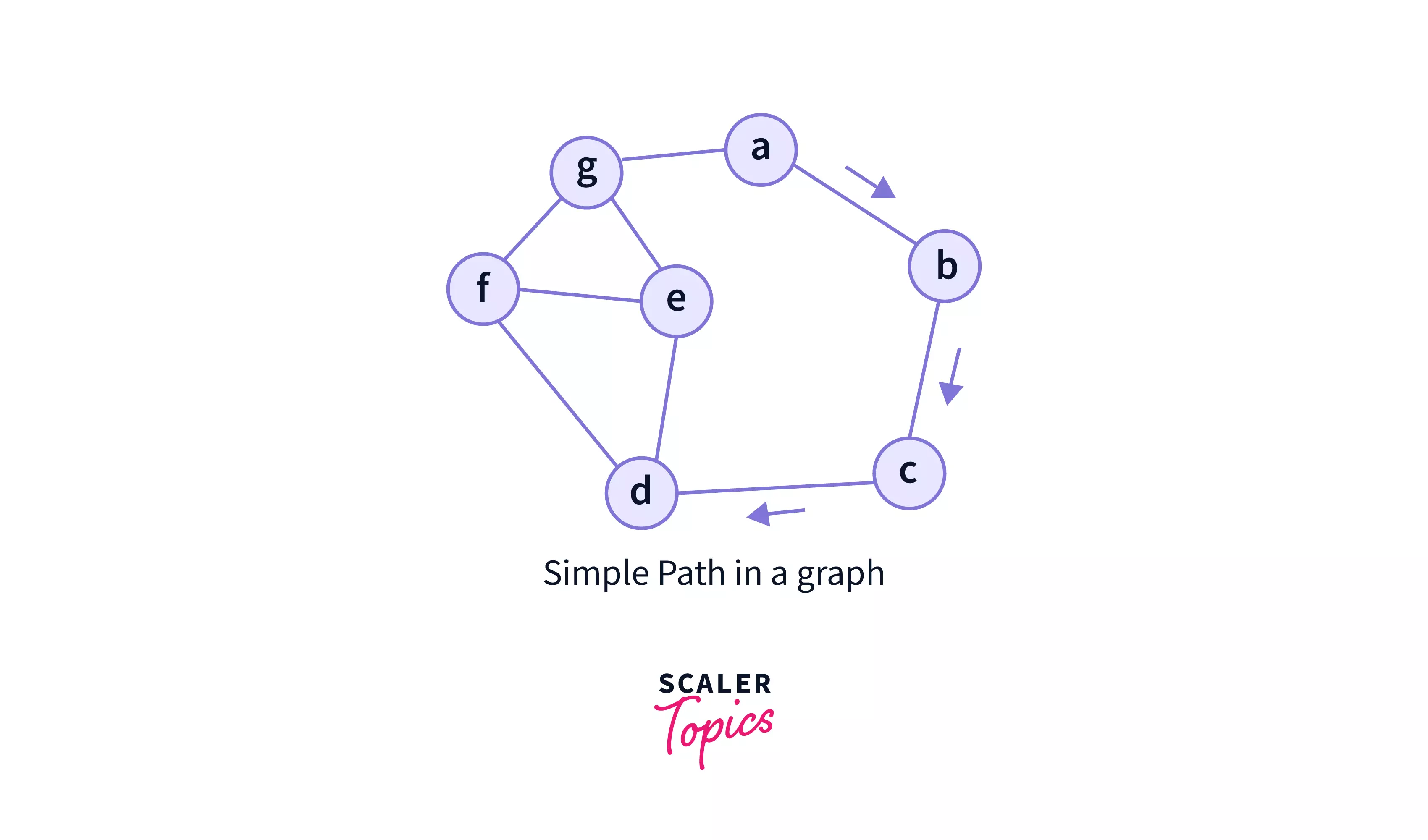
In this example, ${a,b,c,d}$ is a simple path. Because, this graph do not have any loop or cycle and none of the paths point to themselves.

4. Degree of a Node:

Degree of a node is the number of edges connecting the node in the graph. A simple example would be, suppose in facebook, if you have 100 friends then the node that represents you has a degree of 100.

5. Cycle Graph:

A simple graph of ‘n’ nodes(vertices) (n>=3) and n edges forming a cycle of length ‘n’ is called as a cycle graph. In a cycle graph, all the vertices are of degree 2.

Cycle Graph

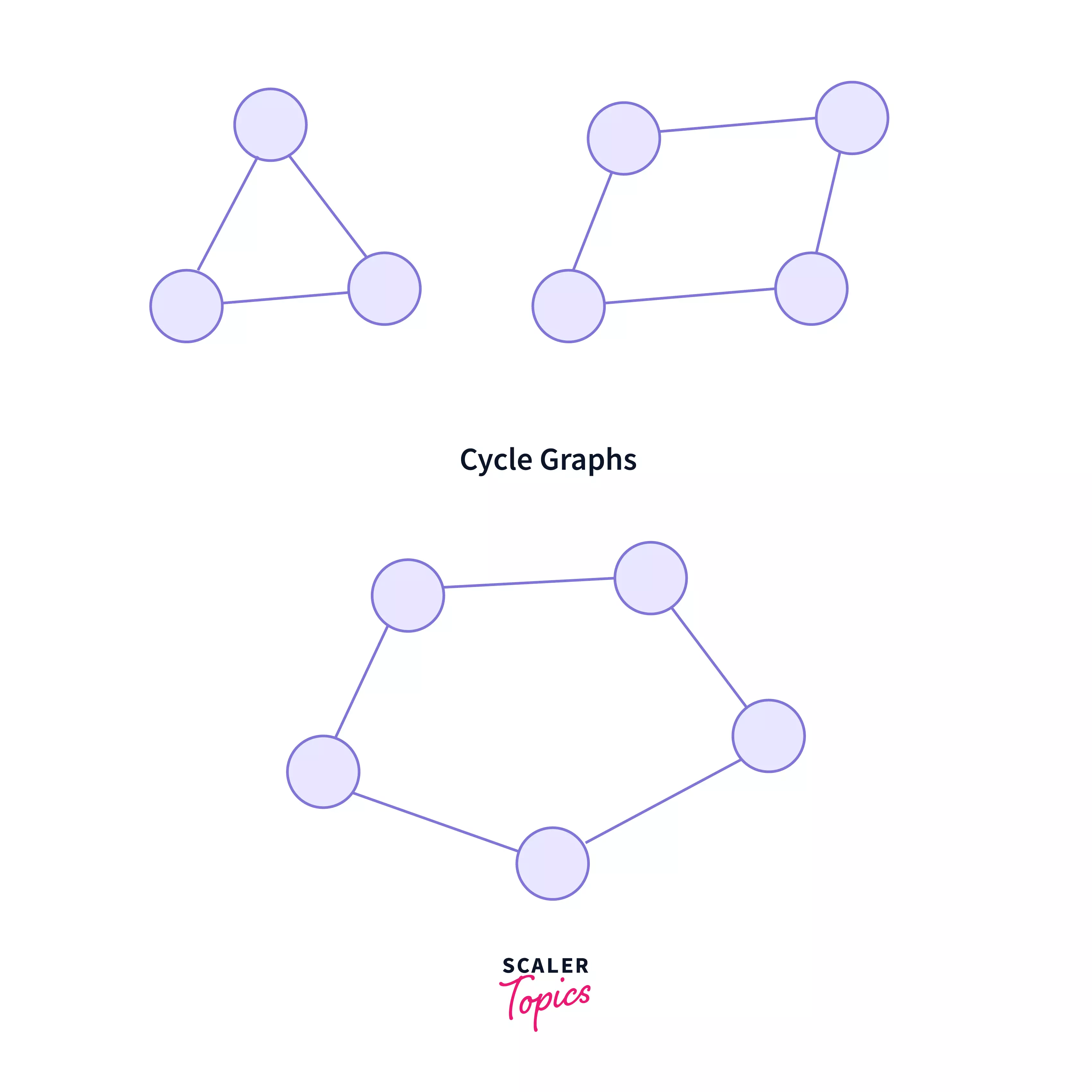
In the above graphs,

Each vertex is having degree 2.
Therefore, they are cycle graphs.

5. Connected Graph:

Connected graph is a graph in which there is an edge or path joining each pair of vertices. So, in a connected graph, it is possible possible to get from one vertex to any other vertex in the graph through a series of edges.

Connected Graph

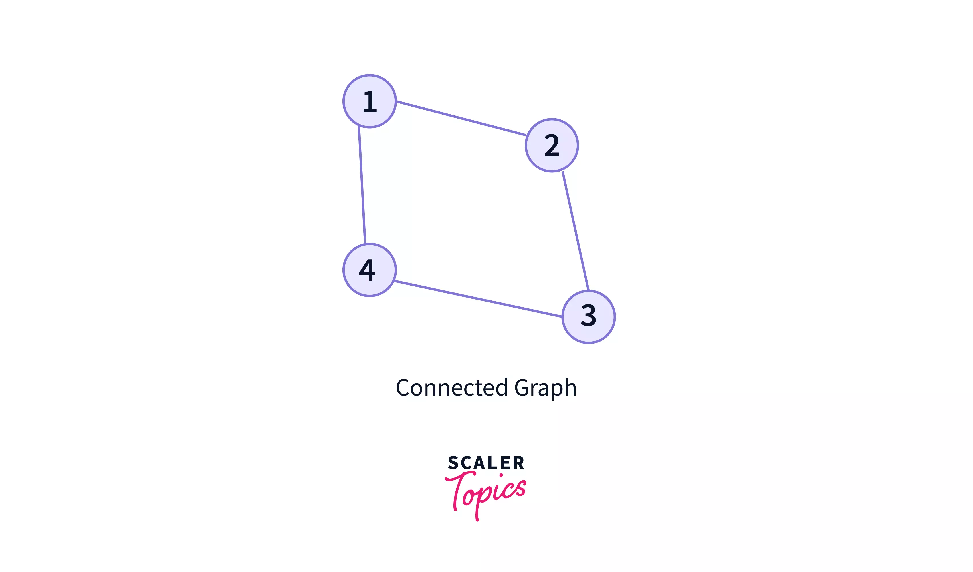
In this graph,

we can visit from any one vertex to any other vertex.
There exists at least one path between every pair of vertices.
There is not a single vertex in a connected graph, which is unreachable(or isolated).
Therefore, it is a connected graph.

6. Complete Graph

In a complete graph, there is an edge between every single pair of node in the graph. Here, every vertex has an edge to all other vertices. It is also known as a full graph.

Key Notes:

A graph in which exactly one edge is present between every pair of vertices is called as a complete graph.
A complete graph of ‘n’ vertices contains exactly $nC_2$ edges.
A complete graph of ‘n’ vertices is represented as $K_n$ .

complete graph

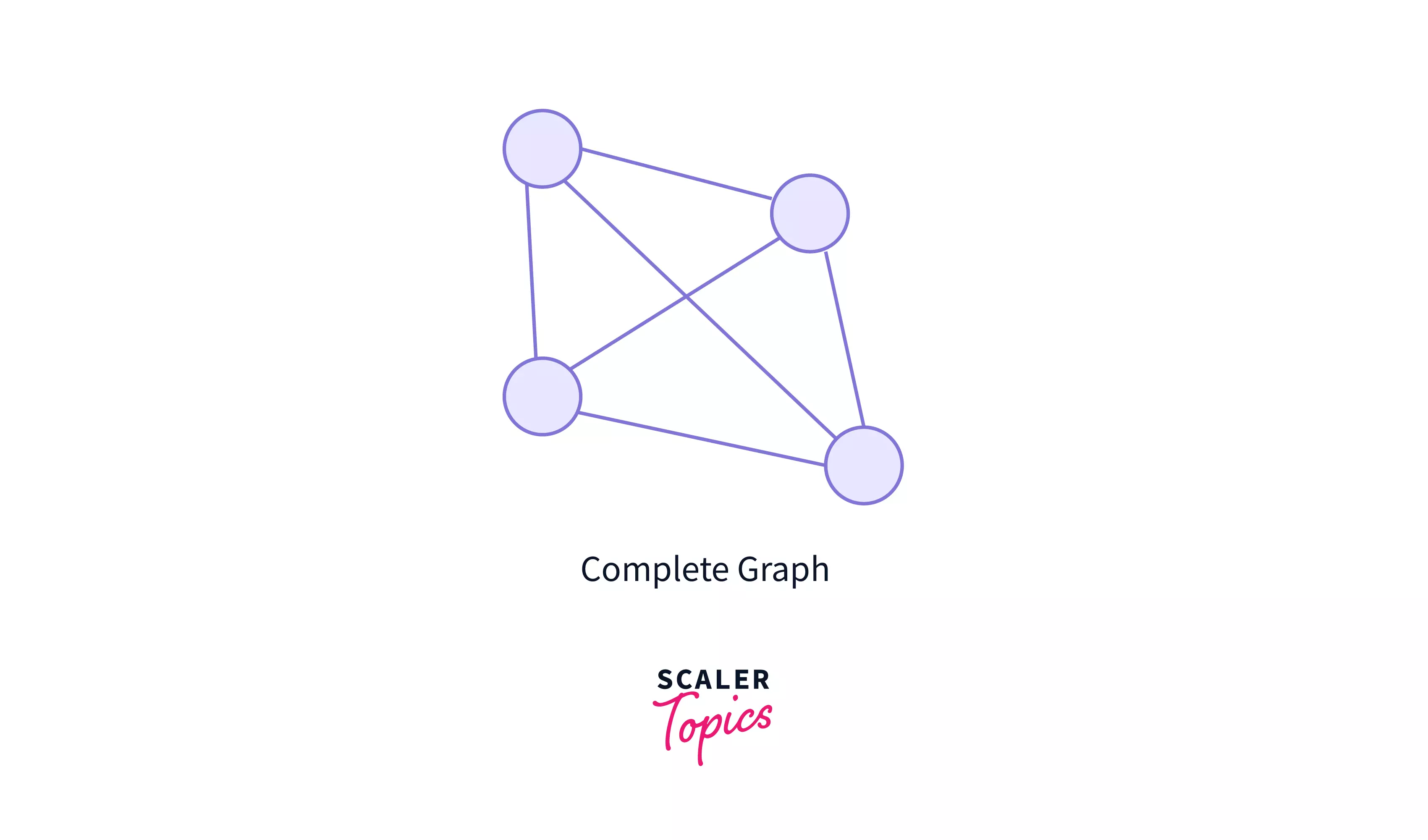
In the above graph,

All the pair of nodes are connected by each other through an edge.
Every complete graph is a connected graph, however, vice versa is not necessary.

Note:

In a Complete graph, the degree of every node is n-1, where, n = number of nodes.

7. Weighted Graph

In weighted graphs, each edge has a value associated with them (called weight). It refers to a simple graph that has weighted edges. The weights are usually used to compute the shortest path in the graph.

Weighted Graph

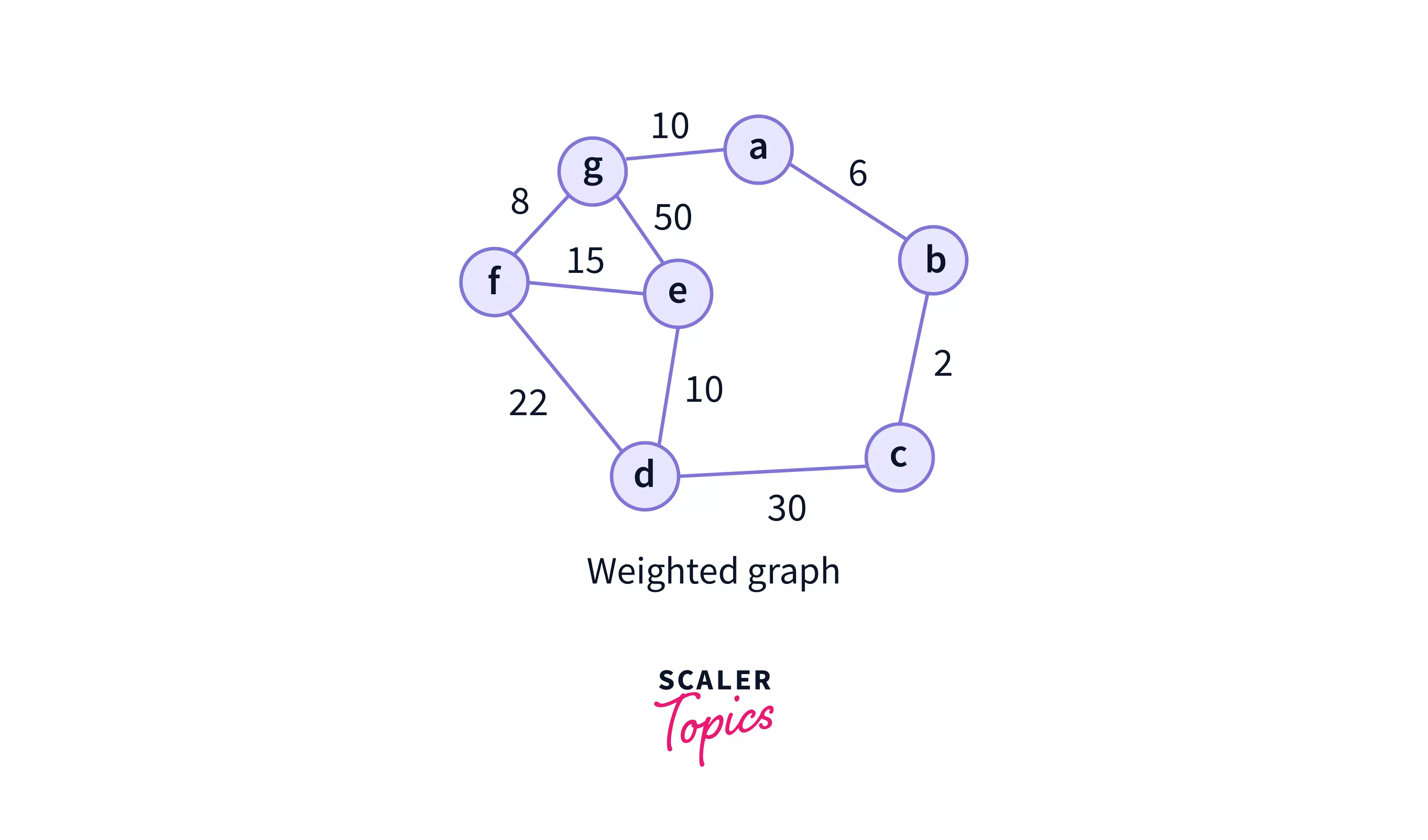
The above graph is a weighted graph, where each edge is associated with a weight. The weights may represent for example, any distance, or time, or the number of connections shared between two users in a social network.

It is not mandatory in a weighted graph that all nodes have distinct weight, i.e. some edges may have same weights.

8. Loop:

A loop (also called a self-loop) is an edge that connects a vertex to itself. It is commonly defined as an edge with both ends as the same vertex.

Although all loops are cycles, not all cycles are loops. Because, cycles do not repeat edges or vertices except for the starting and ending vertex.

Loop in a graph

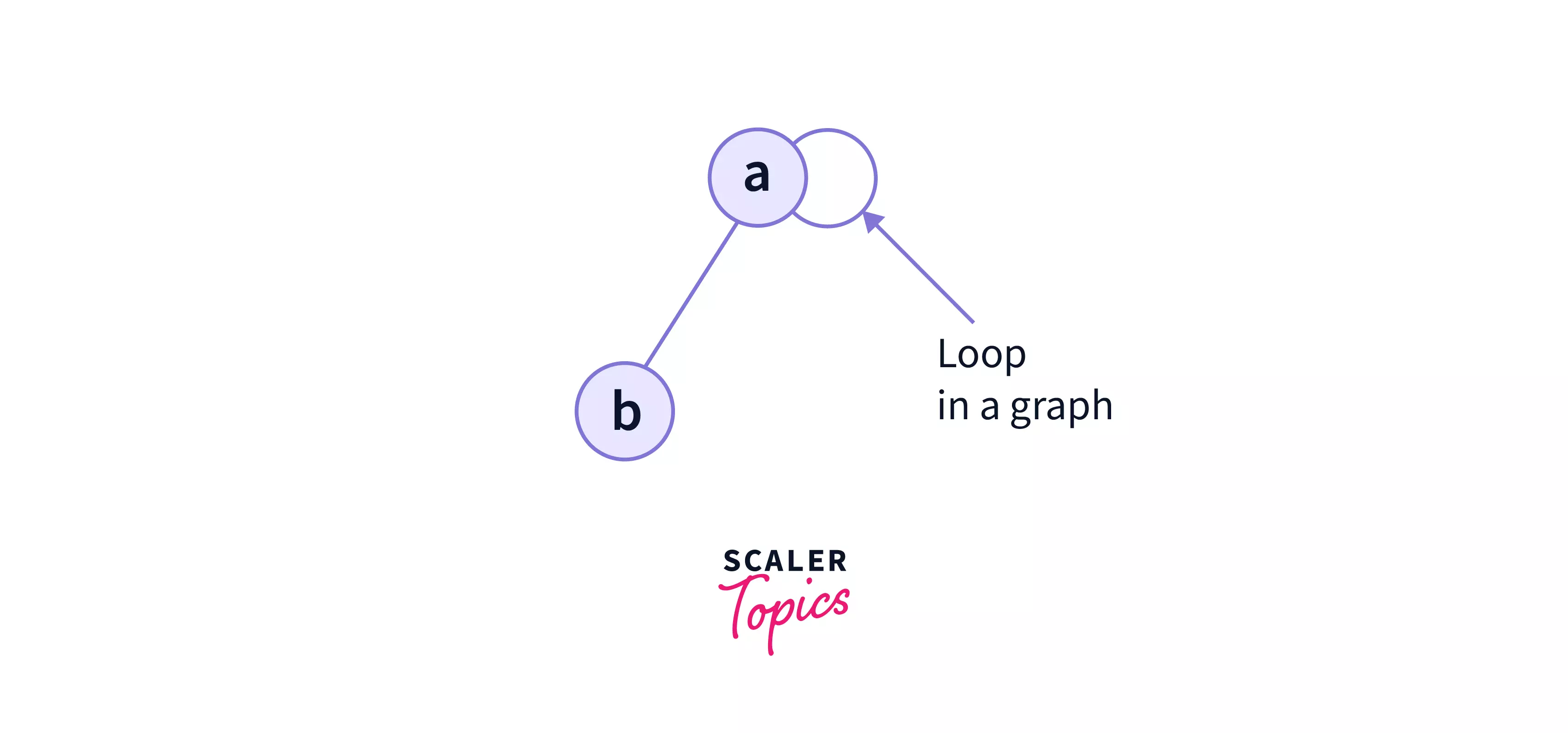
In the above graph,

Ahe node 'a' has a loop in itself.
The staring and ending point of the edge in node 'a' is same.
Hence, there is a loop in the graph.

6. Simple Graph:

A graph having no self loops and no parallel edges in it is called as a simple graph.

Simple Graph

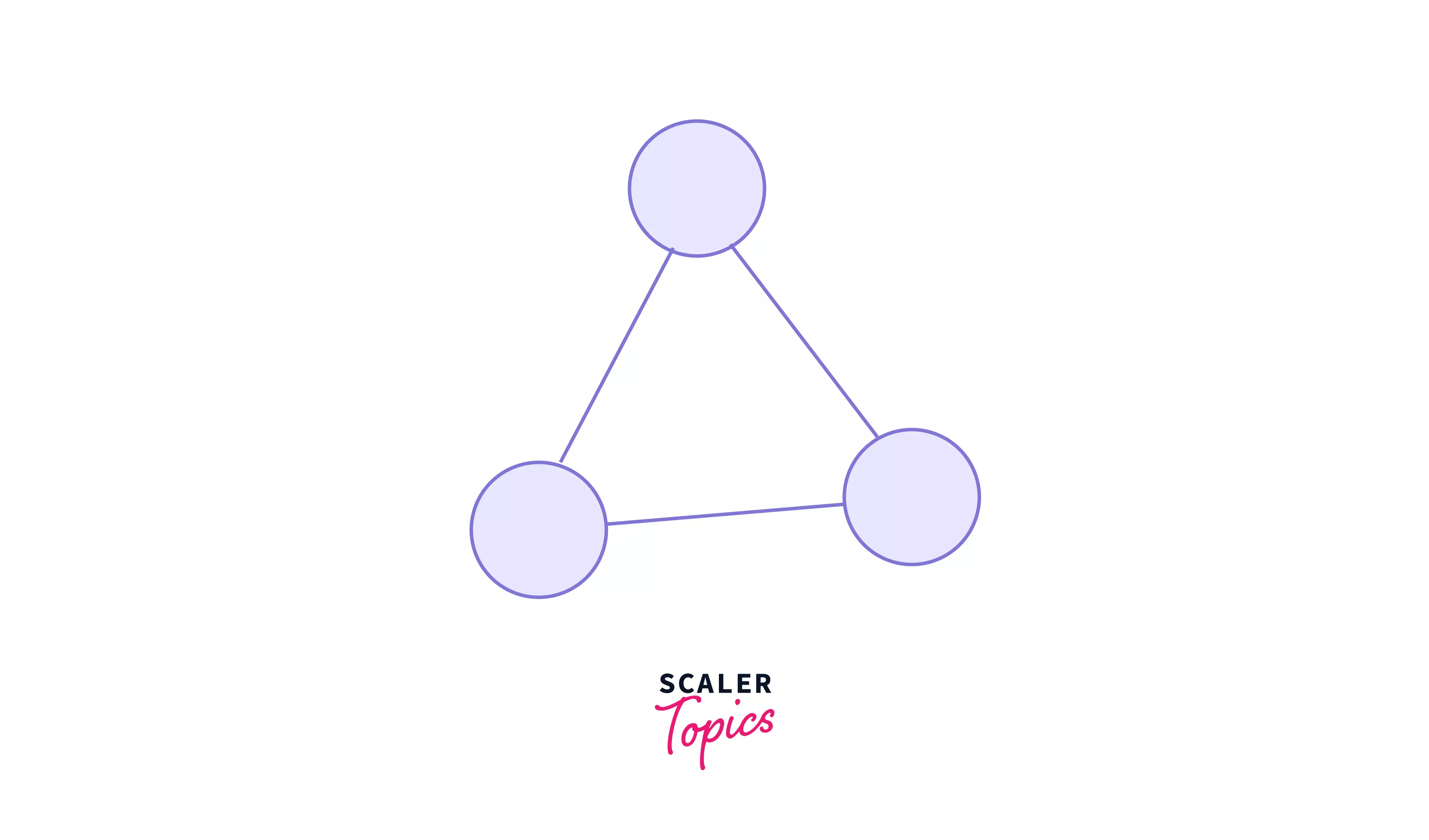
Here,

This graph consists of three vertices and three edges.
There are neither self loops nor parallel edges.
Therefore, it is a simple graph.

Types of Graph

After being familiar with all the terminologies we have in a graph, let us now also look at the types of graphs we have. Graphs are classified based on the characteristics of their edges. There are two types of graphs:

1. Directed Graphs

Directed graphs in graph data structure are the graphs where the edges have directions from one node towards the other node. In Directed Graphs, we can only traverse from one node to another if the edge have a direction pointing to that node.

Directed Graphs

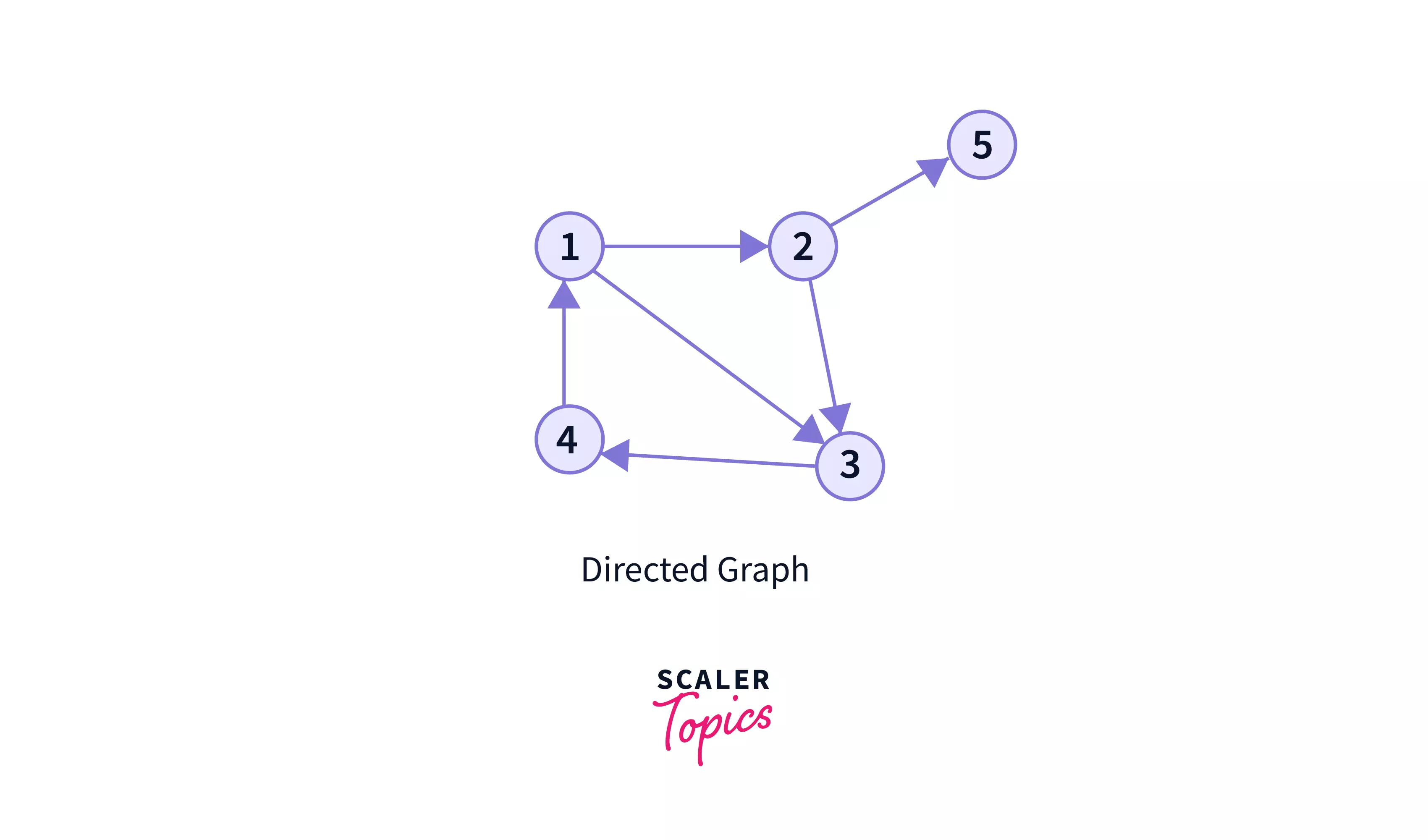
In the above graph, you can see that the edges have arrows that point to a specific direction. So, they are like a one-way street where you can only move from one node to another in the directed edge's direction,and not in the reverse direction.

Suppose, in the shown graph, we can go from node 2 to node 3, but cannot go back to node 2 via node 3. For going back to node 2, we have to find an alternative path like 3 -> 4 -> 1 -> 2 .

Directed graphs are used in many areas. One of the usecase you may think of is a family tree, where there can be only the edge directed from parent to children. So, family tree are directed graphs. It is obvious, because it would not make sense for an individual to simultaneously be the parent and the child of another individual.

2. Undirected Graphs

Undirected graphs have edges that do not have a direction. Hence, the graph can be traversed in either direction.

Undirected Graphs

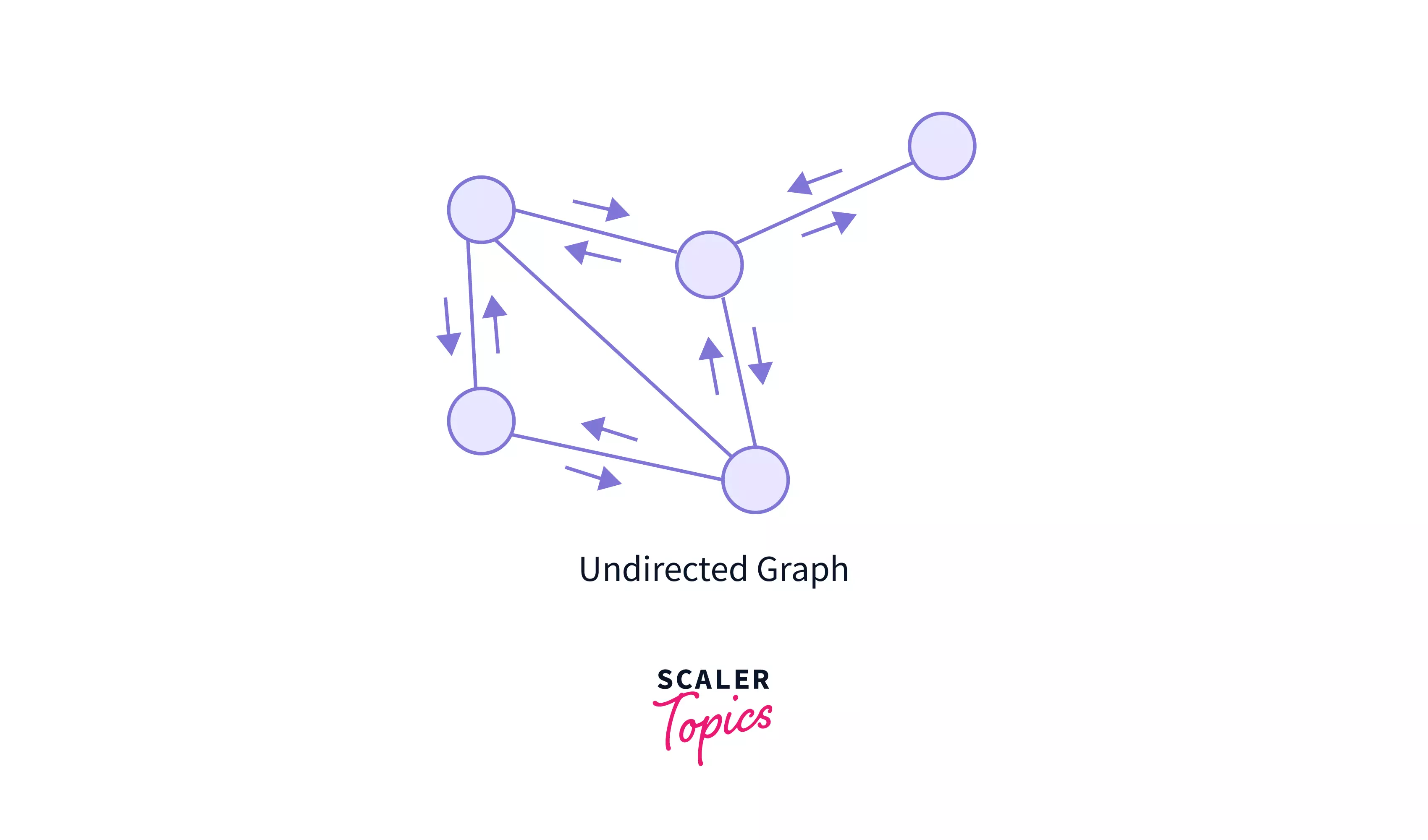
The above graph is undirected. Here, the edges do not point to any direction. We can travel through both the directions, so it is bidirectional. In these graphs, we can reach to one node, from any other node.

You can think of undirected edges as two-way streets. You can go from one node to another and return through that same “path”. Some areas where undirected graphs are very widely used may include the topology of digital social networks, where each friend of someone is that someone’s friend; Suppose Steve is a friend of John, then John too is the friend of Steve. Or, in computer networks, like if one device is connected to another, then the second one is also connected to the first.

Graph Representation

In graph data structure, a graph representation is a technique to store graph into the memory of computer. We can represent a graph in many ways.

The following two are the most commonly used representations of a graph.

Adjacency Matrix
Adjacency List

Let us study about them in details.

Adjacency Matrix

An Adjacency Matrix is a 2D array of size V x V where V is the number of nodes in a graph. It is used to represent a "finite graph", with 0's and 1's. Since, it's size is V x V, it is a square matrix.

The elements of the matrix indicates whether pairs of vertices are adjacent or not in the graph i.e. is there any edge connecting a pair of nodes in the graph.

Let us take an example to simplify the above statements and understand better.
Adjacency Matrix

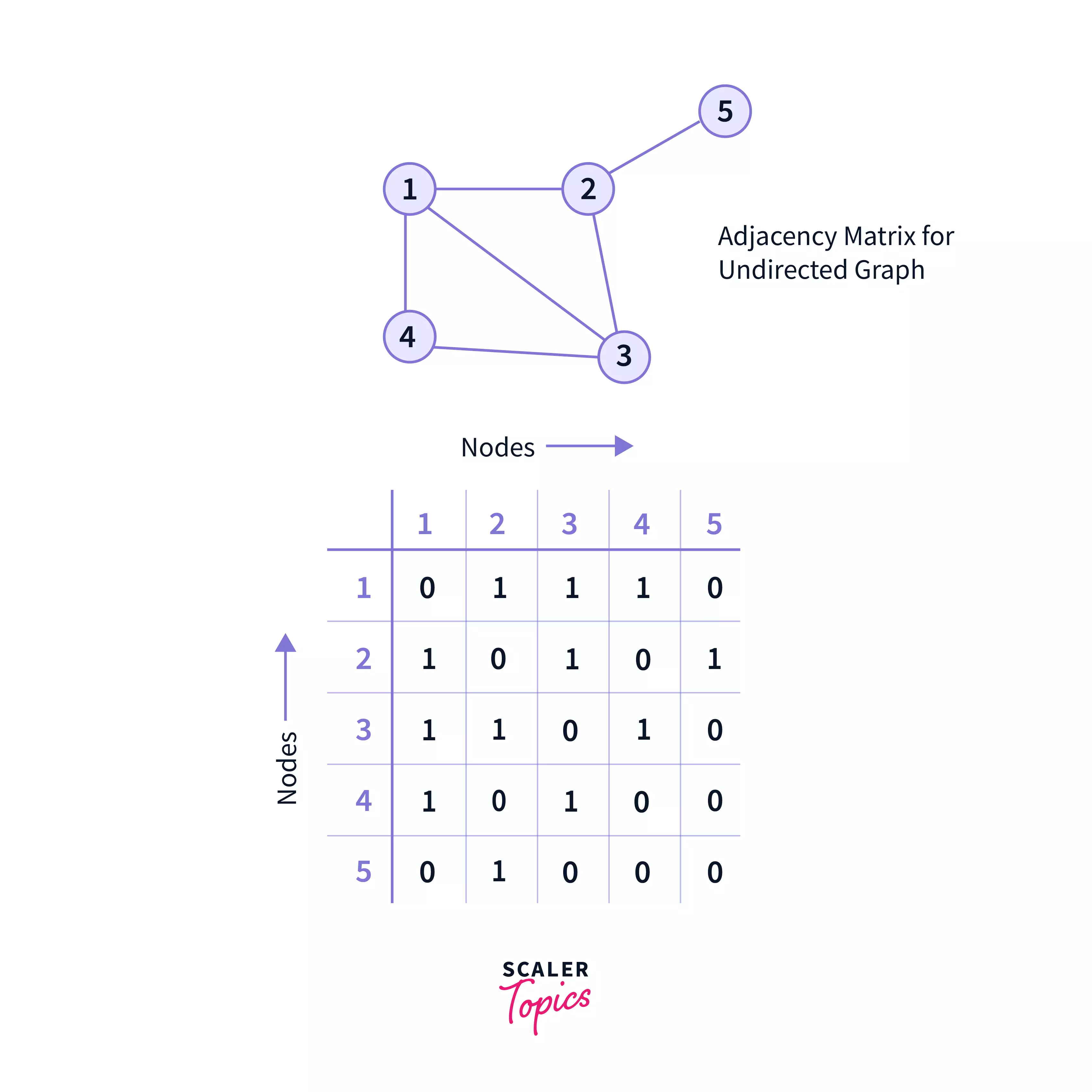
The above example shows the adjacency matrix for the undirected graph. Let us note some important points:

The adjacent matrix's row or column, consists of the nodes or vertices(that is numbered in red, in the above graph).
Each cell in the above matrix is represented as Aij, where i and j are nodes. The value of Aij is either 1 or 0 depending on whether there is an edge from vertex i to vertex j. If there is a node then, Aij= 1, otherwise Aij= 0

Please Note:

Here, we will count the matrix indexes starting from 1, and not from 0, for easy visualization. Please do not get confused. You may consider the nodes indexes marked in red as the matrix index, and read the article.

In the above graph, there is an edge between node 1 & node 2, so in the matrix, we have A[1][2] = 1 and A[2][1] = 1.

If there is no edge between 2 nodes, then that cell in the matrix will contain '0'. For example, there is no edge from node 1 to node 5, so, in the matrix, A[1][5] = 0 and A[5][1] = 0.
Adjacency matrix of an undirected graph is symmetric. Hence, the above graph is symmetric.

The adjacency Matrix for a directed graph also follows the same conventions, expect for, there is a '1' in the matrix if there is an edge pointing from one node to another, say from node A to node B. But vice versa may not be applicable. That is, in a directed graph, if A[i][j] = 1 then A[j][i] may or may not be 1. Adjacency matrix of a directed graph is not symmetric(generally).

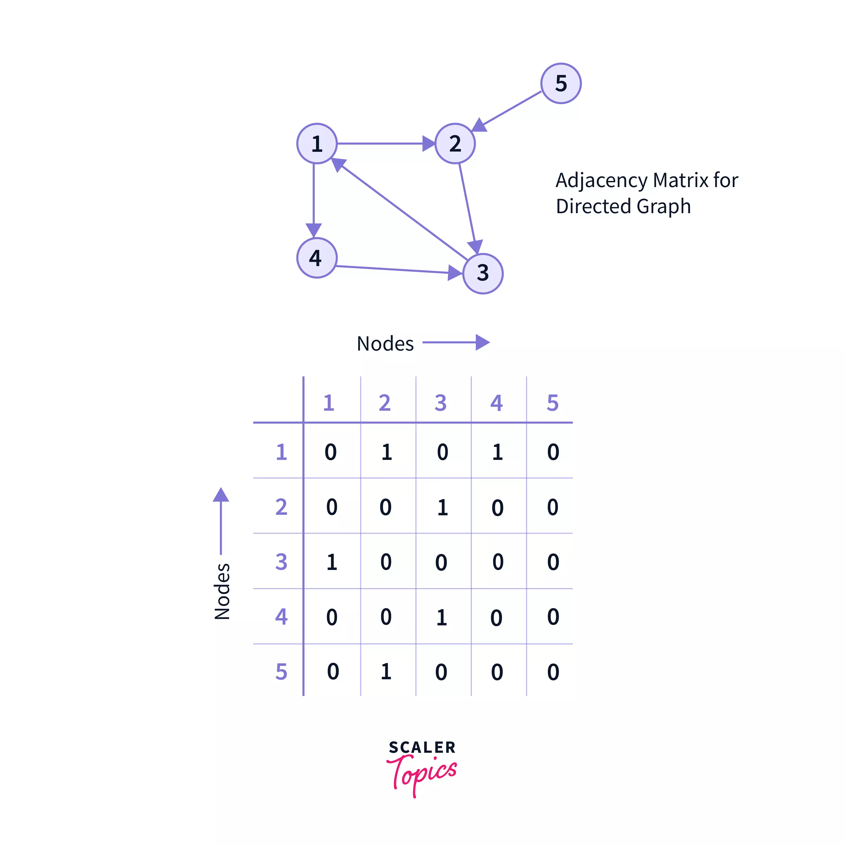
adjacency Matrix for a directed graph

This example clearly shows that, for node 1, we have A[1][2] = 1 but A[2][1] = 0, because we have a directed edge from node 1 to node 2, but there is no edge from node 2 to node 1.

Again, we have a node from node 2 to node 3, so in the matrix, A[2][3] = 1, but A[3][2] = 0, because there is no node from node 3 to node 2.

Adjacency Matrix for Weighted Graphs

If the graph is weighted, then we usually call the matrix as the cost matrix. To store weighted graph using adjacency matrix form, we follow the following steps:

Here each cell at position A[i, j] holds the weight from edge i to j.
If the edge is not present, then it stores infinity or any largest value(which cannot be the weight of any node in the graph).
For same node, the value in the matrix is 0.
Apart from this, the rest of the steps are similar for the adjacency matrix of the graph.

Let us also check some pros and cons for Adjacency Matrix.

Pros of Adjacency Matrix

Adjacency Matrices performs the basic operations like adding an edge, removing an edge, and checking whether there is an edge from node i to node j very efficiently, and in constant time usually.
For dense graphs, where the number of edges are very large, adjacency matrix are the best choice. Because, in big-O terms they don't take up more space, and operations are much faster. Maximum of the cells of matrix are filled because of more number of edges, hence it is very space efficient. If the graph is sparse, then most of the cells are vacant, hence wasting more space.

Cons of Adjacency Matrix

The most notable disadvantage that comes with Adjacency Matrix is the usage of V x V space, where V is the number of vertices. In real life, we do not have so dense connections ,where so many edges will be used. So, the space mostly gets wasted, and hence for sparse graphs with less number of edges Adjacency Lists are always preferred.
Operations like inEdges(to check whether there is an edge directing towards this node) and outEdges(to check whether there is an edge directing out from this node) are expensive in Adjacency Matrix (will study ahead).

Adjacency List

An adjacency list represents a graph as an array of linked lists.
The index of the array represents a node.
Each element in the linked list represents the nodes that are connected to that node by an edge.

Let us take an example for easy visualization --

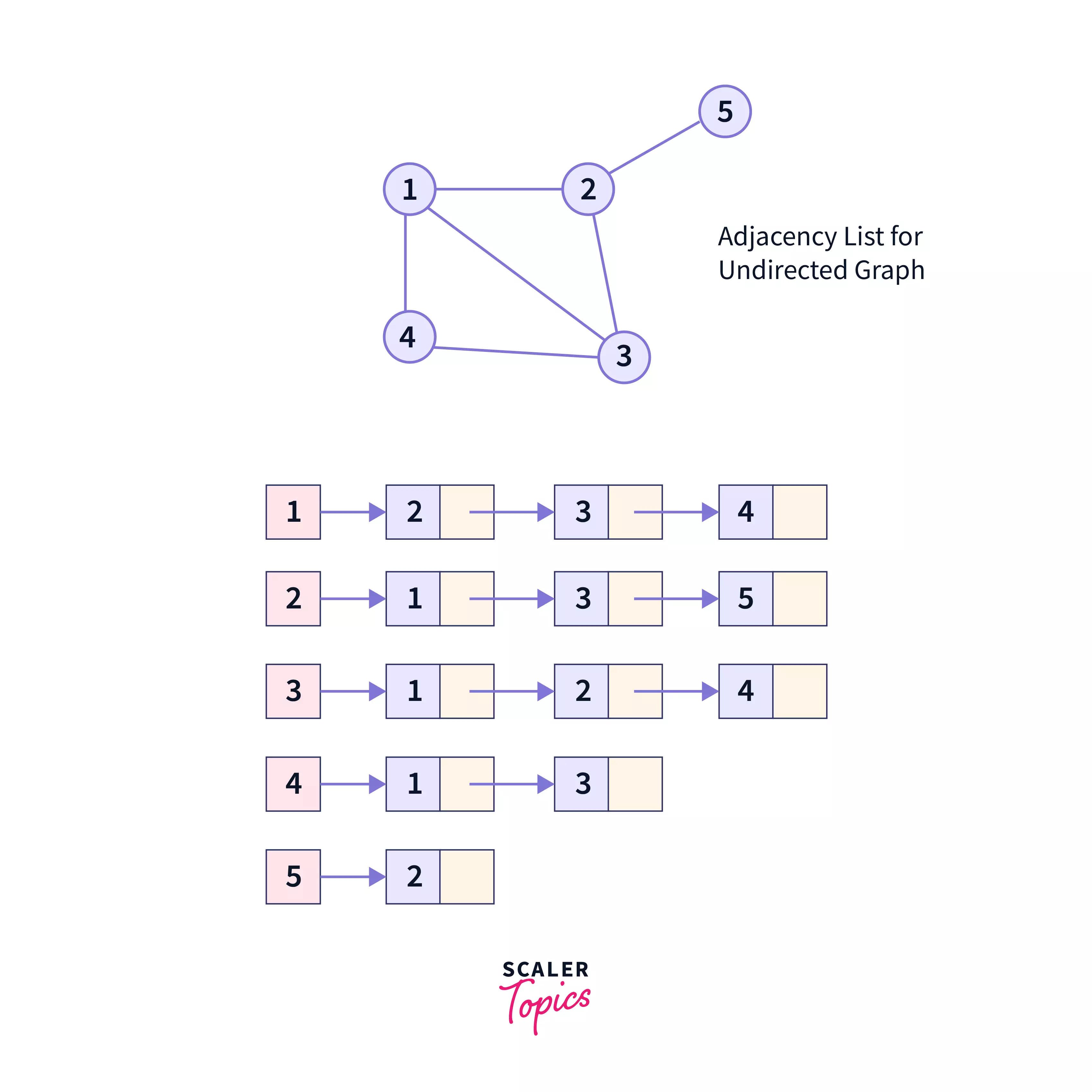
Adjacency List for undirected graph

The graph in our example is undirected and we have represented it using the Adjacency List. Let us look into some important points through this graph:

Here, 1, 2, 3, 4, 5 are the nodes(vertices) and each of them forms an array of linked list with all of its adjacent nodes(vertices).
In the graph, the node 1 has 3 adjacent nodes namely -- node 2, node 3, node 4. So, in the list, the node is linked with 2, 3 & 4.
Node 4 has only 2 adjacent nodes, node 1 & node 3, so it is linked to the nodes 1 and 3 only, in the array of linked list.
The last node in the linked list will point to null.

Adjacency List also follows the same rule in case of directed graph, where the nodes will only be linked to the nodes to whom they have a directed edge(or, to the nodes their outgoing edges are pointing to).

Let us look into few pros & cons for the adjacency list.

Pros of Adjacency list

Since, we only store the value for the edges in the linked lists, the adjacency lists are efficient in terms of storage(for sparse graphs). So, if for some graph we have 1000 edges or 1 edge, we can represent them very efficiently without wasting any space, because we will use list for storage.
Since the adjacency lists are storage efficient, they are useful for storing sparse graphs. Sparse graphs are the graphs, which have the edges much lesser than the number of edges expected.
Adjacency list helps to find all the nodes next to any node easily. Because, a node, points to all the other nodes which are connected to it, hence it becomes very simple to find out all the adjacent nodes.

Cons of Adjacency list

To find any particular node in an adjacency list, we need to explore all the connected nodes. So, usually it is slower as compared to finding a node in an adjacency matrix.
It is not a good option for dense graphs because, we will unnecessarily be storing so many edges in the linked list and hence it will neither be memory efficient, nor time efficient in terms of certain operations(like search or peek).

Graph Operations

These are the few basic graphs operations mentioned below:

Add Vertex: Here, we simply add a vertex(node) in a graph. It need not be connected to any other vertex(node) through an edge.

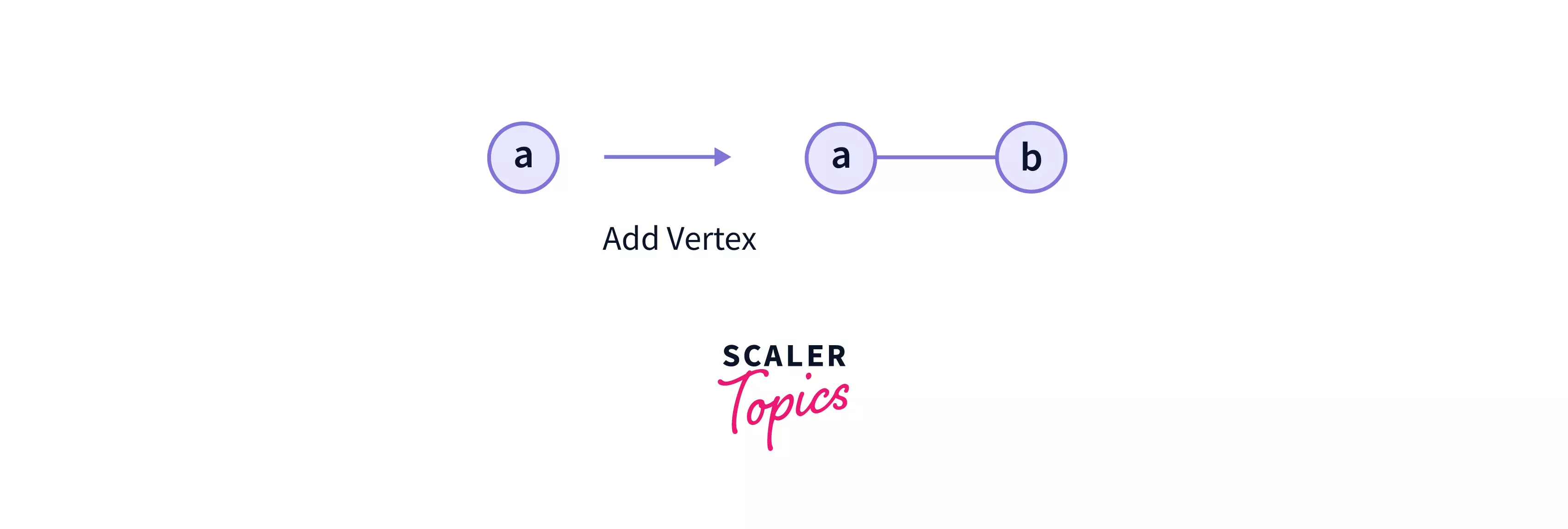
In the above example, we have added the vertex 'a' into the graph.

Remove Vertex: We remove a vertex from the graph. But, before removing the vertex, we also remove all the edges associated with that vertex. It means, while removing a vertex, we remove any edge that is outgoing or ingoing to that vertex.

remove vertex in a graph

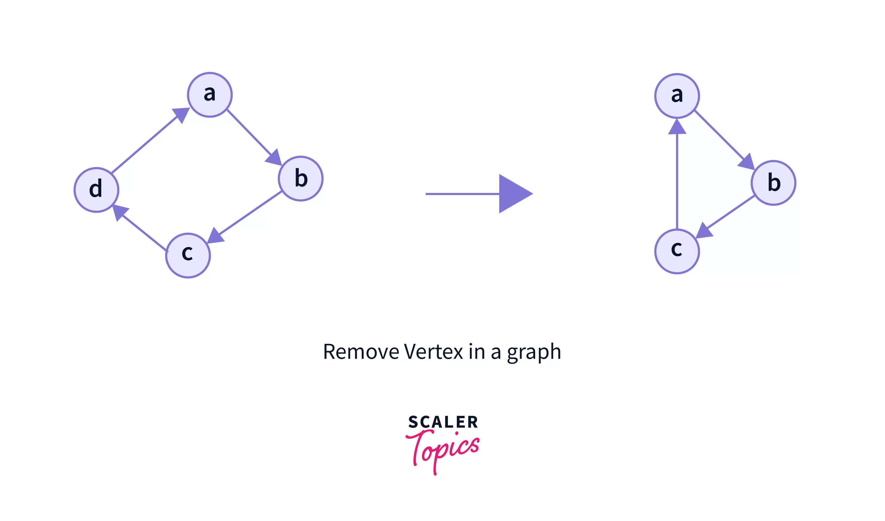
In the above example, we have removed the vertex 'd' from the graph.

Add edge: This operation is responsible for adding an edge between a pair of vertices.

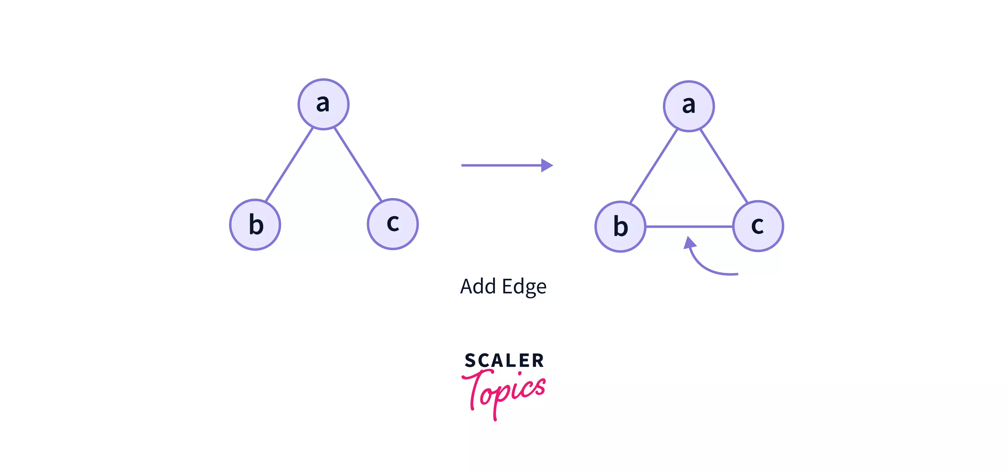
In the above example, we have added the edge between vertex 'b' and vertex 'c' in the graph.

Removing edge: It involves removing an edge from a graph. If all the edges from a particular vertex(node) is removed, then that vertex(node) becomes an isolated vertex.

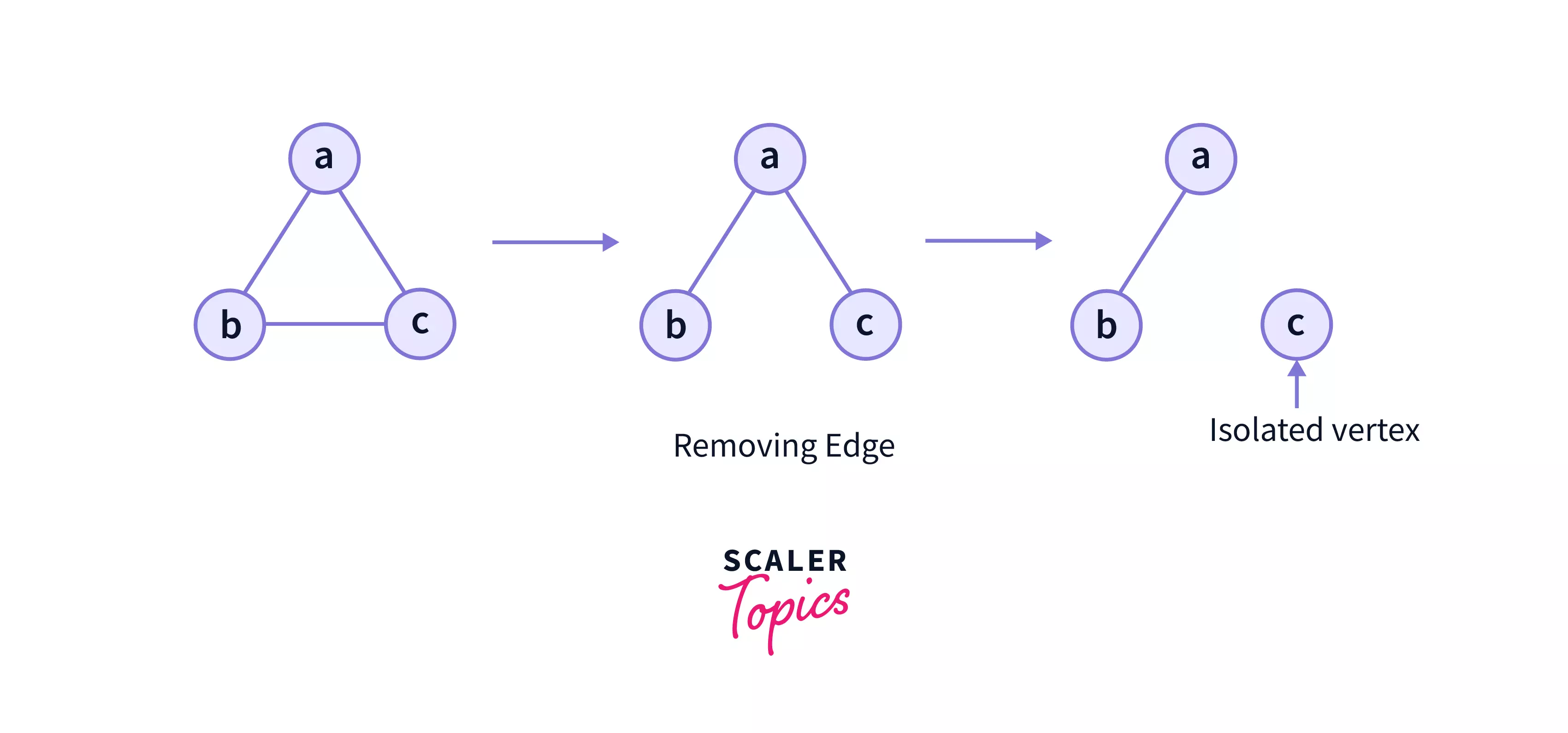
In the above example, we have removed the edge between vertex b and vertex c from the graph.
After that, we have also removed the edge between vertex a and vertex c, so vertex c becomes an isolated edge.

Has Edge: This operation checks for an edge in the graph. It checks, whether an edge is present or not in the graph data structure.
Graph traversal: It includes traversing all the edges of a graph.

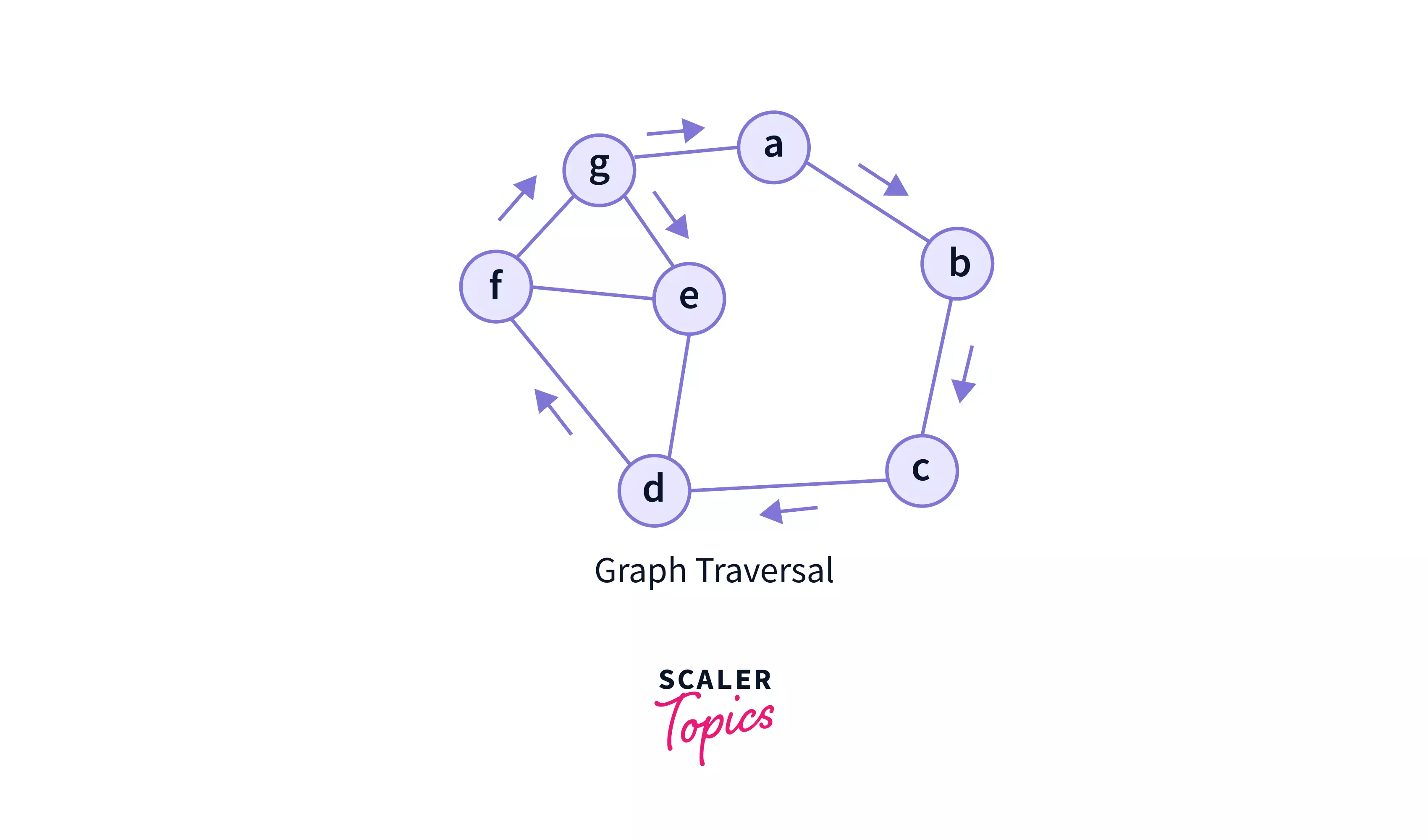
In the above graph, we have traversed through all the edges in the graph.

Display vertex: It helps to display one or more vertices of the graph.

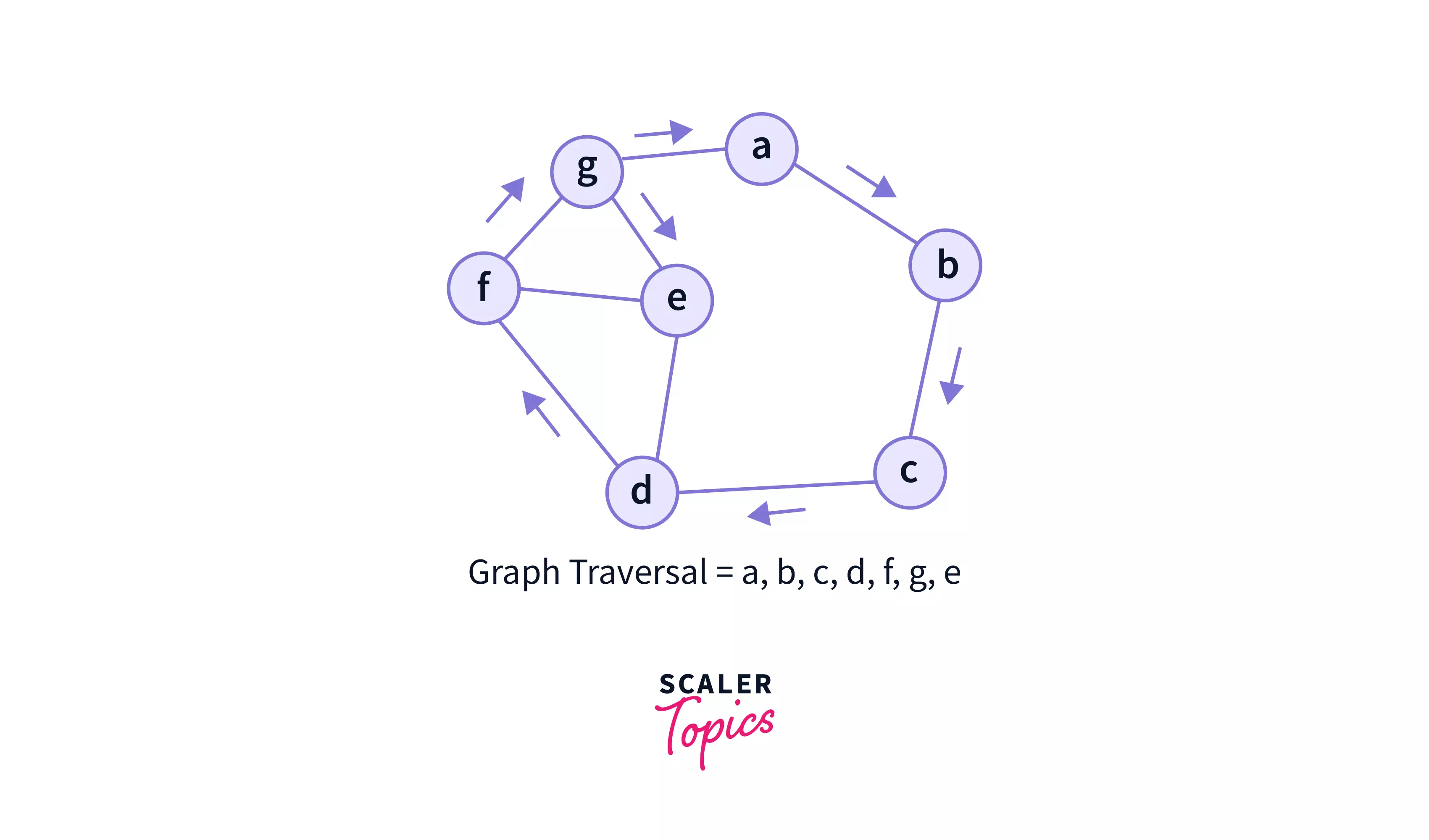
In the above graph, we have traversed and displayed all the vertices of the graph.

Practical Applications of Graph

GPS systems and Google Maps use graphs to find the shortest path from one destination to another.
The Google Search algorithm uses graphs to determine the relevance of search results.
World Wide Web is the biggest graph. All the links and hyperlinks are the nodes and their interconnection is the edges. This is why we can open one webpage from the other.
Social Networks like facebook, twitter, etc. use graphs to represent connections between users.
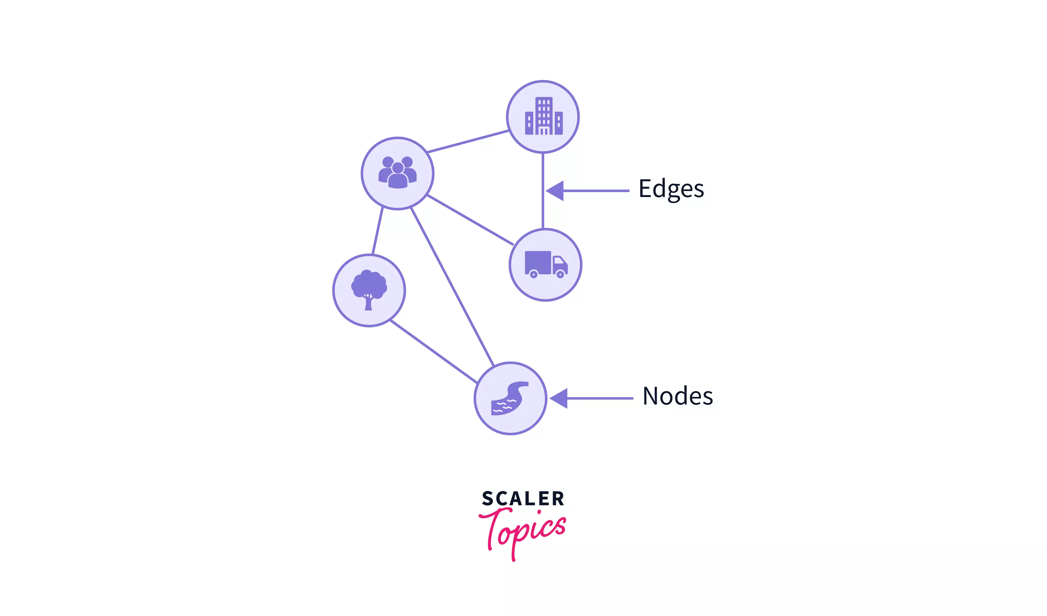
The nodes we represent in our graphs can be considered as the buildings, people, group, landmarks or anything in general , whereas the edges are the paths connecting them.

Just like in the below image, egdes are the roadways / path connecting the nodes(like people, buildings, transports, etc). edges and nodes

Conclusion

Let us recap what we learnt throughout this article:

A Graph data structure is a collection of nodes that have data and are connected to other nodes through edges.
Weighted graphs are the graph in Data Structure in which the edges are given some weight or value based on the type of graph we are representing
Unweighted graphs are the graph in Data Structure which are not associated with any weight or value. By default their weight or value is considered as 1.
Directed graphs are the graph in Data Structure where the edges have some direction.
Undirected graphs are the graph in Data Structure which do not have any particular direction.
Adjacency Matrix representation of graphs are done through 2D arrays or matrices.
Adjacency List are the array of linked list and are meant to store the edges connected to a node.
We can perform various operations on graph in Data Structure like adding/ removing node, adding/ removing edge, graph traversals, displaying nodes, inedge, out-edge, etc.
There are major real-life implementations of graph in Data Structures like they are used in social networks, google maps, google search engine, GPS, etc.

See More

Graph Transversal in Data Structures